Data analysis course notes (V) common statistical methods, data and spelling, index and composite index

pandas Common statistical methods

Data sources ：
https://www.kaggle.com/damianpanek/sunday-eda/data

# coding=utf-8
import pandas as pd
import numpy as np

file_path = "IMDB-Movie-Data.csv"
df = pd.read_csv(file_path)

# print(df.info())

print(df.head(1))

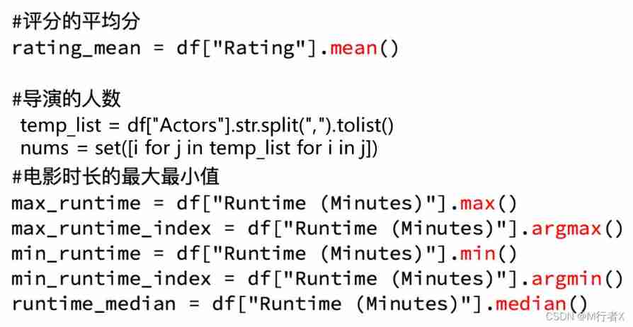
# Get the average score 
print(df["Rating"].mean())

# The number of Directors 
# print(len(set(df["Director"].tolist())))
print(len(df["Director"].unique()))

# Get the number of actors 
temp_actors_list = df["Actors"].str.split(", ").tolist()
actors_list = [i for j in temp_actors_list for i in j]
actors_num = len(set(actors_list))
print(actors_num)

# coding=utf-8
import pandas as pd
from matplotlib import pyplot as plt
file_path = "./IMDB-Movie-Data.csv"

df = pd.read_csv(file_path)
# print(df.head(1))
# print(df.info())

#rating,runtime Distribution situation 
# Select graphics , Histogram 
# Prepare the data 
runtime_data = df["Rating"].values

max_runtime = runtime_data.max()
min_runtime = runtime_data.min()

# Count groups 
print(max_runtime-min_runtime)
num_bin = (max_runtime-min_runtime)//0.5


# Set the size of the graph 
plt.figure(figsize=(20,8),dpi=80)
plt.hist(runtime_data,num_bin)

_x = [min_runtime]
i = min_runtime
while i<=max_runtime+0.5:
    i = i+0.5
    _x.append(i)

plt.xticks(_x)

plt.show()

import numpy as np
from matplotlib import pyplot as plt

runtime_data = np.array([8.1, 7.0, 7.3, 7.2, 6.2, 6.1, 8.3, 6.4, 7.1, 7.0, 7.5, 7.8, 7.9, 7.7, 6.4, 6.6, 8.2, 6.7, 8.1, 8.0, 6.7, 7.9, 6.7, 6.5, 5.3, 6.8, 8.3, 4.7, 6.2, 5.9, 6.3, 7.5, 7.1, 8.0, 5.6, 7.9, 8.6, 7.6, 6.9, 7.1, 6.3, 7.5, 2.7, 7.2, 6.3, 6.7, 7.3, 5.6, 7.1, 3.7, 8.1, 5.8, 5.6, 7.2, 9.0, 7.3, 7.2, 7.4, 7.0, 7.5, 6.7, 6.8, 6.5, 4.1, 8.5, 7.7, 7.4, 8.1, 7.5, 7.2, 5.9, 7.1, 7.5, 6.8, 8.1, 7.1, 8.1, 8.3, 7.3, 5.3, 8.8, 7.9, 8.2, 8.1, 7.2, 7.0, 6.4, 7.8, 7.8, 7.4, 8.1, 7.0, 8.1, 7.1, 7.4, 7.4, 8.6, 5.8, 6.3, 8.5, 7.0, 7.0, 8.0, 7.9, 7.3, 7.7, 5.4, 6.3, 5.8, 7.7, 6.3, 8.1, 6.1, 7.7, 8.1, 5.8, 6.2, 8.8, 7.2, 7.4, 6.7, 6.7, 6.0, 7.4, 8.5, 7.5, 5.7, 6.6, 6.4, 8.0, 7.3, 6.0, 6.4, 8.5, 7.1, 7.3, 8.1, 7.3, 8.1, 7.1, 8.0, 6.2, 7.8, 8.2, 8.4, 8.1, 7.4, 7.6, 7.6, 6.2, 6.4, 7.2, 5.8, 7.6, 8.1, 4.7, 7.0, 7.4, 7.5, 7.9, 6.0, 7.0, 8.0, 6.1, 8.0, 5.2, 6.5, 7.3, 7.3, 6.8, 7.9, 7.9, 5.2, 8.0, 7.5, 6.5, 7.6, 7.0, 7.4, 7.3, 6.7, 6.8, 7.0, 5.9, 8.0, 6.0, 6.3, 6.6, 7.8, 6.3, 7.2, 5.6, 8.1, 5.8, 8.2, 6.9, 6.3, 8.1, 8.1, 6.3, 7.9, 6.5, 7.3, 7.9, 5.7, 7.8, 7.5, 7.5, 6.8, 6.7, 6.1, 5.3, 7.1, 5.8, 7.0, 5.5, 7.8, 5.7, 6.1, 7.7, 6.7, 7.1, 6.9, 7.8, 7.0, 7.0, 7.1, 6.4, 7.0, 4.8, 8.2, 5.2, 7.8, 7.4, 6.1, 8.0, 6.8, 3.9, 8.1, 5.9, 7.6, 8.2, 5.8, 6.5, 5.9, 7.6, 7.9, 7.4, 7.1, 8.6, 4.9, 7.3, 7.9, 6.7, 7.5, 7.8, 5.8, 7.6, 6.4, 7.1, 7.8, 8.0, 6.2, 7.0, 6.0, 4.9, 6.0, 7.5, 6.7, 3.7, 7.8, 7.9, 7.2, 8.0, 6.8, 7.0, 7.1, 7.7, 7.0, 7.2, 7.3, 7.6, 7.1, 7.0, 6.0, 6.1, 5.8, 5.3, 5.8, 6.1, 7.5, 7.2, 5.7, 7.7, 7.1, 6.6, 5.7, 6.8, 7.1, 8.1, 7.2, 7.5, 7.0, 5.5, 6.4, 6.7, 6.2, 5.5, 6.0, 6.1, 7.7, 7.8, 6.8, 7.4, 7.5, 7.0, 5.2, 5.3, 6.2, 7.3, 6.5, 6.4, 7.3, 6.7, 7.7, 6.0, 6.0, 7.4, 7.0, 5.4, 6.9, 7.3, 8.0, 7.4, 8.1, 6.1, 7.8, 5.9, 7.8, 6.5, 6.6, 7.4, 6.4, 6.8, 6.2, 5.8, 7.7, 7.3, 5.1, 7.7, 7.3, 6.6, 7.1, 6.7, 6.3, 5.5, 7.4, 7.7, 6.6, 7.8, 6.9, 5.7, 7.8, 7.7, 6.3, 8.0, 5.5, 6.9, 7.0, 5.7, 6.0, 6.8, 6.3, 6.7, 6.9, 5.7, 6.9, 7.6, 7.1, 6.1, 7.6, 7.4, 6.6, 7.6, 7.8, 7.1, 5.6, 6.7, 6.7, 6.6, 6.3, 5.8, 7.2, 5.0, 5.4, 7.2, 6.8, 5.5, 6.0, 6.1, 6.4, 3.9, 7.1, 7.7, 6.7, 6.7, 7.4, 7.8, 6.6, 6.1, 7.8, 6.5, 7.3, 7.2, 5.6, 5.4, 6.9, 7.8, 7.7, 7.2, 6.8, 5.7, 5.8, 6.2, 5.9, 7.8, 6.5, 8.1, 5.2, 6.0, 8.4, 4.7, 7.0, 7.4, 6.4, 7.1, 7.1, 7.6, 6.6, 5.6, 6.3, 7.5, 7.7, 7.4, 6.0, 6.6, 7.1, 7.9, 7.8, 5.9, 7.0, 7.0, 6.8, 6.5, 6.1, 8.3, 6.7, 6.0, 6.4, 7.3, 7.6, 6.0, 6.6, 7.5, 6.3, 7.5, 6.4, 6.9, 8.0, 6.7, 7.8, 6.4, 5.8, 7.5, 7.7, 7.4, 8.5, 5.7, 8.3, 6.7, 7.2, 6.5, 6.3, 7.7, 6.3, 7.8, 6.7, 6.7, 6.6, 8.0, 6.5, 6.9, 7.0, 5.3, 6.3, 7.2, 6.8, 7.1, 7.4, 8.3, 6.3, 7.2, 6.5, 7.3, 7.9, 5.7, 6.5, 7.7, 4.3, 7.8, 7.8, 7.2, 5.0, 7.1, 5.7, 7.1, 6.0, 6.9, 7.9, 6.2, 7.2, 5.3, 4.7, 6.6, 7.0, 3.9, 6.6, 5.4, 6.4, 6.7, 6.9, 5.4, 7.0, 6.4, 7.2, 6.5, 7.0, 5.7, 7.3, 6.1, 7.2, 7.4, 6.3, 7.1, 5.7, 6.7, 6.8, 6.5, 6.8, 7.9, 5.8, 7.1, 4.3, 6.3, 7.1, 4.6, 7.1, 6.3, 6.9, 6.6, 6.5, 6.5, 6.8, 7.8, 6.1, 5.8, 6.3, 7.5, 6.1, 6.5, 6.0, 7.1, 7.1, 7.8, 6.8, 5.8, 6.8, 6.8, 7.6, 6.3, 4.9, 4.2, 5.1, 5.7, 7.6, 5.2, 7.2, 6.0, 7.3, 7.2, 7.8, 6.2, 7.1, 6.4, 6.1, 7.2, 6.6, 6.2, 7.9, 7.3, 6.7, 6.4, 6.4, 7.2, 5.1, 7.4, 7.2, 6.9, 8.1, 7.0, 6.2, 7.6, 6.7, 7.5, 6.6, 6.3, 4.0, 6.9, 6.3, 7.3, 7.3, 6.4, 6.6, 5.6, 6.0, 6.3, 6.7, 6.0, 6.1, 6.2, 6.7, 6.6, 7.0, 4.9, 8.4, 7.0, 7.5, 7.3, 5.6, 6.7, 8.0, 8.1, 4.8, 7.5, 5.5, 8.2, 6.6, 3.2, 5.3, 5.6, 7.4, 6.4, 6.8, 6.7, 6.4, 7.0, 7.9, 5.9, 7.7, 6.7, 7.0, 6.9, 7.7, 6.6, 7.1, 6.6, 5.7, 6.3, 6.5, 8.0, 6.1, 6.5, 7.6, 5.6, 5.9, 7.2, 6.7, 7.2, 6.5, 7.2, 6.7, 7.5, 6.5, 5.9, 7.7, 8.0, 7.6, 6.1, 8.3, 7.1, 5.4, 7.8, 6.5, 5.5, 7.9, 8.1, 6.1, 7.3, 7.2, 5.5, 6.5, 7.0, 7.1, 6.6, 6.5, 5.8, 7.1, 6.5, 7.4, 6.2, 6.0, 7.6, 7.3, 8.2, 5.8, 6.5, 6.6, 6.2, 5.8, 6.4, 6.7, 7.1, 6.0, 5.1, 6.2, 6.2, 6.6, 7.6, 6.8, 6.7, 6.3, 7.0, 6.9, 6.6, 7.7, 7.5, 5.6, 7.1, 5.7, 5.2, 5.4, 6.6, 8.2, 7.6, 6.2, 6.1, 4.6, 5.7, 6.1, 5.9, 7.2, 6.5, 7.9, 6.3, 5.0, 7.3, 5.2, 6.6, 5.2, 7.8, 7.5, 7.3, 7.3, 6.6, 5.7, 8.2, 6.7, 6.2, 6.3, 5.7, 6.6, 4.5, 8.1, 5.6, 7.3, 6.2, 5.1, 4.7, 4.8, 7.2, 6.9, 6.5, 7.3, 6.5, 6.9, 7.8, 6.8, 4.6, 6.7, 6.4, 6.0, 6.3, 6.6, 7.8, 6.6, 6.2, 7.3, 7.4, 6.5, 7.0, 4.3, 7.2, 6.2, 6.2, 6.8, 6.0, 6.6, 7.1, 6.8, 5.2, 6.7, 6.2, 7.0, 6.3, 7.8, 7.6, 5.4, 7.6, 5.4, 4.6, 6.9, 6.8, 5.8, 7.0, 5.8, 5.3, 4.6, 5.3, 7.6, 1.9, 7.2, 6.4, 7.4, 5.7, 6.4, 6.3, 7.5, 5.5, 4.2, 7.8, 6.3, 6.4, 7.1, 7.1, 6.8, 7.3, 6.7, 7.8, 6.3, 7.5, 6.8, 7.4, 6.8, 7.1, 7.6, 5.9, 6.6, 7.5, 6.4, 7.8, 7.2, 8.4, 6.2, 7.1, 6.3, 6.5, 6.9, 6.9, 6.6, 6.9, 7.7, 2.7, 5.4, 7.0, 6.6, 7.0, 6.9, 7.3, 5.8, 5.8, 6.9, 7.5, 6.3, 6.9, 6.1, 7.5, 6.8, 6.5, 5.5, 7.7, 3.5, 6.2, 7.1, 5.5, 7.1, 7.1, 7.1, 7.9, 6.5, 5.5, 6.5, 5.6, 6.8, 7.9, 6.2, 6.2, 6.7, 6.9, 6.5, 6.6, 6.4, 4.7, 7.2, 7.2, 6.7, 7.5, 6.6, 6.7, 7.5, 6.1, 6.4, 6.3, 6.4, 6.8, 6.1, 4.9, 7.3, 5.9, 6.1, 7.1, 5.9, 6.8, 5.4, 6.3, 6.2, 6.6, 4.4, 6.8, 7.3, 7.4, 6.1, 4.9, 5.8, 6.1, 6.4, 6.9, 7.2, 5.6, 4.9, 6.1, 7.8, 7.3, 4.3, 7.2, 6.4, 6.2, 5.2, 7.7, 6.2, 7.8, 7.0, 5.9, 6.7, 6.3, 6.9, 7.0, 6.7, 7.3, 3.5, 6.5, 4.8, 6.9, 5.9, 6.2, 7.4, 6.0, 6.2, 5.0, 7.0, 7.6, 7.0, 5.3, 7.4, 6.5, 6.8, 5.6, 5.9, 6.3, 7.1, 7.5, 6.6, 8.5, 6.3, 5.9, 6.7, 6.2, 5.5, 6.2, 5.6, 5.3])
max_runtime = runtime_data.max()
min_runtime = runtime_data.min()
print(min_runtime,max_runtime)

# Set unequal group spacing ,hist What you get in the method will be a left closed and right open interval [1.9,3.5)
num_bin_list = [1.9,3.5]
i=3.5
while i<=max_runtime:
    i += 0.5
    num_bin_list.append(i)
print(num_bin_list)

# Set the size of the graph 
plt.figure(figsize=(20,8),dpi=80)
plt.hist(runtime_data,num_bin_list)

#xticks Let the previous group spacing correspond to 
plt.xticks(num_bin_list)

plt.show()

# coding=utf-8
import pandas as pd
from matplotlib import pyplot as plt
import numpy as np
file_path = "./IMDB-Movie-Data.csv"

df = pd.read_csv(file_path)
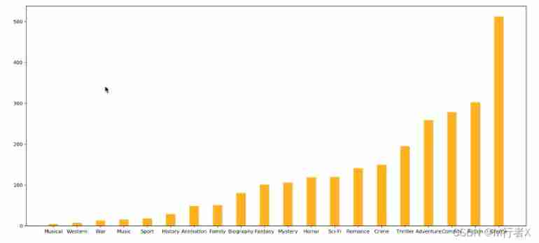
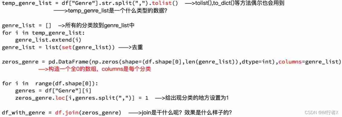
print(df["Genre"].head(3))
# List of statistical classifications 
temp_list = df["Genre"].str.split(",").tolist()  #[[],[],[]]

genre_list = list(set([i for j in temp_list for i in j]))

# The structure is all 0 Array of 
zeros_df = pd.DataFrame(np.zeros((df.shape[0],len(genre_list))),columns=genre_list)
# print(zeros_df)

# Assign a value to the location of each movie occurrence category 1
for i in range(df.shape[0]):
    #zeros_df.loc[0,["Sci-fi","Mucical"]] = 1
    zeros_df.loc[i,temp_list[i]] = 1

# print(zeros_df.head(3))

# Count the number and number of films in each category 
genre_count = zeros_df.sum(axis=0)
print(genre_count)

# Sort 
genre_count = genre_count.sort_values()
_x = genre_count.index
_y = genre_count.values
# drawing 
plt.figure(figsize=(20,8),dpi=80)
plt.bar(range(len(_x)),_y,width=0.4,color="orange")
plt.xticks(range(len(_x)),_x)
plt.show()

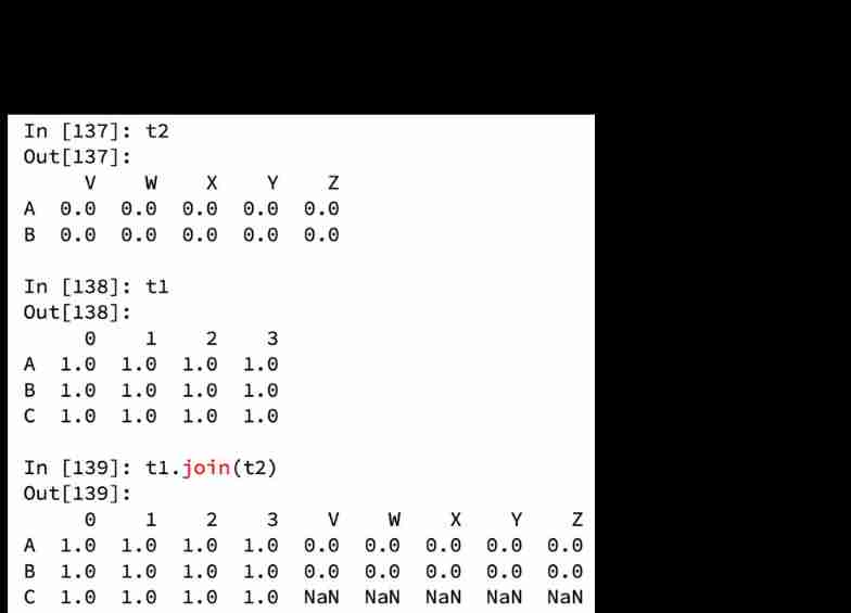
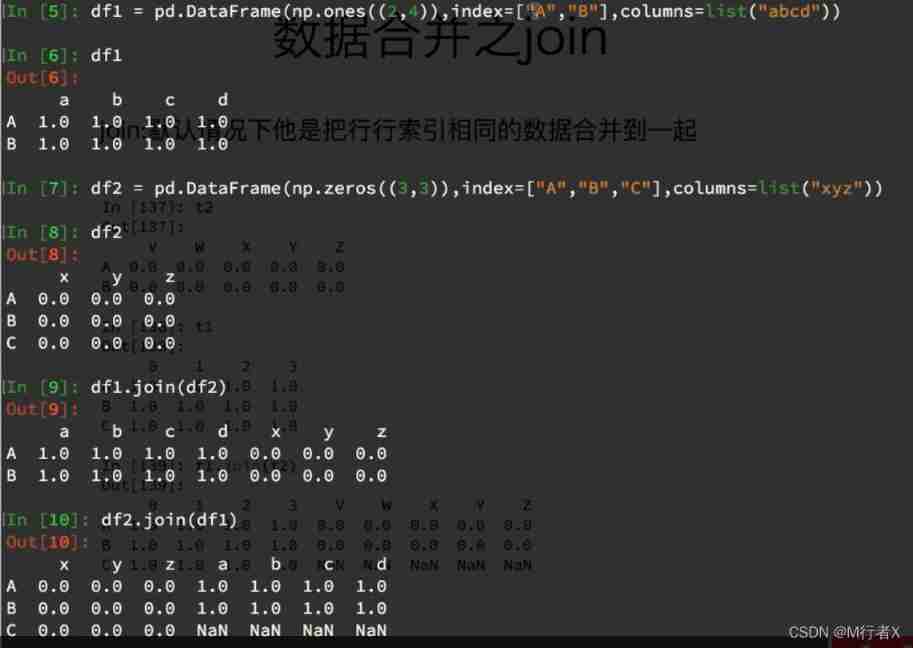
Data merging Join

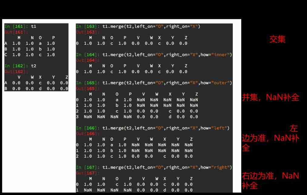
Data merging Merge

Group and aggregate

Data sources ：
https://www.kaggle.com/starbucks/store-locations/data

# coding=utf-8
import pandas as pd
import numpy as np

file_path = "./starbucks_store_worldwide.csv"

df = pd.read_csv(file_path)
# print(df.head(1))
# print(df.info())
# grouped = df.groupby(by="Country")
# print(grouped)

#DataFrameGroupBy
# It can be traversed 
# for i,j in grouped:
# print(i)
# print("-"*100)
# print(j,type(j))
# print("*"*100)
# df[df["Country"]="US"]
# Call aggregate method 


# country_count = grouped["Brand"].count()
# print(country_count["US"])
# print(country_count["CN"])

# Count the number of stores in each province of China 
# china_data = df[df["Country"] =="CN"]
#
# grouped = china_data.groupby(by="State/Province").count()["Brand"]
#
# print(grouped)

# Data is grouped according to multiple criteria , return Series
# grouped = df["Brand"].groupby(by=[df["Country"],df["State/Province"]]).count()
# print(grouped)
# print(type(grouped))

# Data is grouped according to multiple criteria , return DataFrame
grouped1 = df[["Brand"]].groupby(by=[df["Country"],df["State/Province"]]).count()
# grouped2= df.groupby(by=[df["Country"],df["State/Province"]])[["Brand"]].count()
# grouped3 = df.groupby(by=[df["Country"],df["State/Province"]]).count()[["Brand"]]

print(grouped1,type(grouped1))
# print("*"*100)
# print(grouped2,type(grouped2))
# print("*"*100)
#
# print(grouped3,type(grouped3))

# Index methods and properties 
print(grouped1.index)

Index and composite index

Composite index

# coding=utf-8
import pandas as pd
from matplotlib import pyplot as plt

file_path = "./starbucks_store_worldwide.csv"

df = pd.read_csv(file_path)

# Use matplotlib Show the top of the total number of stores 10 The country 
# Prepare the data 
data1 = df.groupby(by="Country").count()["Brand"].sort_values(ascending=False)[:10]

_x = data1.index
_y = data1.values

# drawing 
plt.figure(figsize=(20,8),dpi=80)

plt.bar(range(len(_x)),_y)

plt.xticks(range(len(_x)),_x)

plt.show()

# coding=utf-8
import pandas as pd
from matplotlib import pyplot as plt
from matplotlib import font_manager

my_font = font_manager.FontProperties(fname="/Library/Fonts/Songti.ttc")

file_path = "./starbucks_store_worldwide.csv"

df = pd.read_csv(file_path)
df = df[df["Country"]=="CN"]

# Use matplotlib Show the top of the total number of stores 10 The country 
# Prepare the data 
data1 = df.groupby(by="City").count()["Brand"].sort_values(ascending=False)[:25]

_x = data1.index
_y = data1.values

# drawing 
plt.figure(figsize=(20,12),dpi=80)

# plt.bar(range(len(_x)),_y,width=0.3,color="orange")
plt.barh(range(len(_x)),_y,height=0.3,color="orange")

plt.yticks(range(len(_x)),_x,fontproperties=my_font)

plt.show()

Receipt source ：
https://www.kaggle.com/zygmunt/goodbooks-10k

# coding=utf-8
import pandas as pd
from matplotlib import pyplot as plt


file_path = "./books.csv"

df = pd.read_csv(file_path)
# print(df.head(2))
#
# print(df.info())

# data1 = df[pd.notnull(df["original_publication_year"])]
#
# grouped = data1.groupby(by="original_publication_year").count()["title"]


# Average score of books in different years 
# Remove original_publication_year In the column nan The line of 
data1 = df[pd.notnull(df["original_publication_year"])]

grouped = data1["average_rating"].groupby(by=data1["original_publication_year"]).mean()

# print(grouped)

_x = grouped.index
_y = grouped.values

# drawing 
plt.figure(figsize=(20,8),dpi=80)
plt.plot(range(len(_x)),_y)
print(len(_x))

plt.xticks(list(range(len(_x)))[::10],_x[::10].astype(int),rotation=45)
plt.show()

Data sources ：
https://www.kaggle.com/mchirico/montcoalert/data

# coding=utf-8
import pandas as pd
import numpy as np
from matplotlib import pyplot as plt


df = pd.read_csv("./911.csv")

print(df.head(5))
# Get categories 
# print()df["title"].str.split(": ")
temp_list = df["title"].str.split(": ").tolist()
cate_list = list(set([i[0] for i in temp_list]))
print(cate_list)

# The structure is all 0 Array of 
zeros_df = pd.DataFrame(np.zeros((df.shape[0],len(cate_list))),columns=cate_list)

# assignment 
for cate in cate_list:
    zeros_df[cate][df["title"].str.contains(cate)] = 1
    # break
# print(zeros_df)

sum_ret = zeros_df.sum(axis=0)
print(sum_ret)

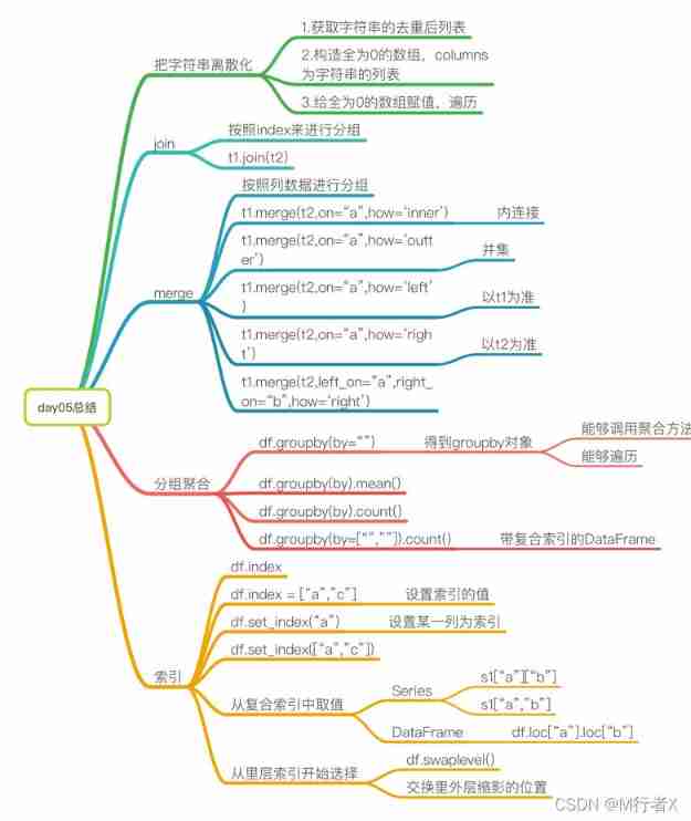
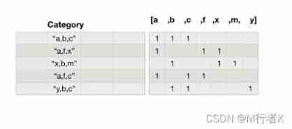
####  String discretization for statistics 
  -  Get the list after classification and de duplication 
  -  The structure is all 0 Of DataFrame, The shape is （ Number of rows of data , Length of classification list ）, Column index is the list after classification and de duplication 
  -  Traverse the raw data , Yes, it's all 0 Of df assignment 
    - zeros_df.loc[i,["T","M"]] = 1
  -  Sum by column 

#### join
  -  Merge by row index 

#### merge
  -  Sum and merge according to a certain column 

  [
  [1,2,3],
  [4,5,6]
  ]
  [
  [10,2,31],
  [43,52,62]
  ]
  ret:  Left connection 
  [
  [1,2,3,10,2,31],
  [4,5,6,nan,nan,nan]
  ]

  ret:  Internal connection 
  [
  [1,2,3,10,2,31]
  ]

  ret:  External connection 
  [
  [1,2,3,10,2,31]
  [4,5,6,nan,nan,nan]
  [nan,nan,nan,43,52,62]
  ]

  ret:  The right connection 
  [
  [1,2,3,10,2,31]
  [nan,nan,nan,43,52,62]
  ]


####  Grouping and aggregation of data 
  - groupby(by="").count()

  - groupby(by=["",""]).count() ---> Returns the df

  -  Can the iteration 




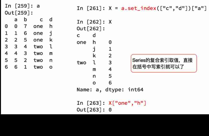
####  Relevant knowledge points of index 
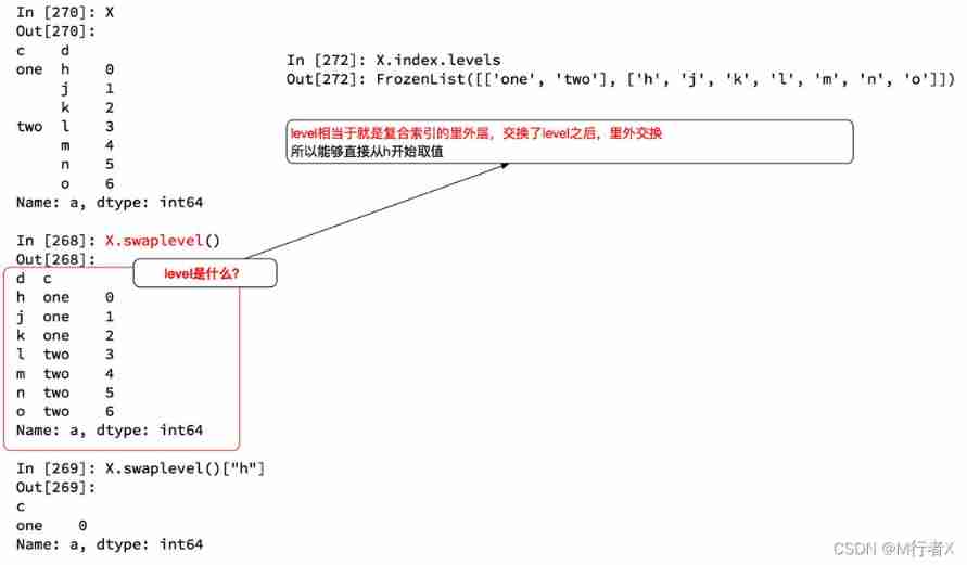
  - df.index
  - df.index = []
  - df.set_index(“a”) # Take a column as an index 
  - df.set_index([“a”,"b"]) # Take some columns as indexes 

  - series
    - `s1["a"]["b"]`
    - `s1["a","b"]`

  - DataFrame
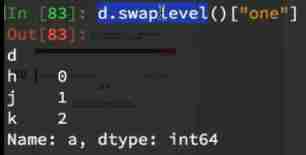
    - `df.loc["a"].loc["b"]`

  -  Choose from the inner layer 
    - df.swaplevel()