当前位置:网站首页>Probability is not yet. Look at statistical learning methods -- Chapter 4, naive Bayesian method
Probability is not yet. Look at statistical learning methods -- Chapter 4, naive Bayesian method
2022-07-02 09:12:00 【Qigui】
Author's brief introduction : The most important part of the whole building is the foundation , The foundation is unstable , The earth trembled and the mountains swayed . And to learn technology, we should lay a solid foundation , Pay attention to me , Take you to firm the foundation of the neighborhood of each plate .
Blog home page : Qigui's blog
Included column :《 Statistical learning method 》 The second edition —— Personal notes
From the south to the North , Don't miss it , Miss this article ,“ wonderful ” May miss you la
Triple attack( Three strikes in a row ):Comment,Like and Collect—>Attention
List of articles
brief introduction
Naive Bayes is a classification method based on Bayes theorem and independent assumption of characteristic conditions . For a given training dataset , First, the joint probability distribution of input and output is learned based on the assumption of characteristic conditional independence ; And then based on this model , A new instance of a given input x, The maximum posterior probability output is obtained by using Bayesian theorem y.
Naive Bayes does not directly learn the joint probability distribution of input and output , It's done by learning the class's prior probability and class's conditional probability .
Naive Bayes method includes the learning and classification of naive Bayes method 、 Parameter estimation algorithm of naive Bayesian method .
1、 Full probability formula and Bayes theorem
- probability : event X The possibility of occurrence is called X Probability of occurrence , use ~P(X) To express
- Prior probability : Judge the probability of the event through experience , Or when this probability distribution has been determined before the field test or sampling
- Posterior probability : On the premise of known results , The probability of inferring the cause
- Conditional probability : When events Y When it has happened , event X The possibility of happening , Called in Y Under the condition of X Conditional probability of occurrence , use ~P(X|Y) Express
A priori probability distribution :
P ( Y = c k ) , k = 1 , 2 , . . . , k P(Y=c_{k}),k=1,2,...,k P(Y=ck),k=1,2,...,k
Conditional probability distribution :
P ( X = x ∣ Y = c k ) = P ( X 1 = x 1 , . . . , X n = x n ∣ Y = c k ) , k = 1 , 2 , . . . , k P(X=x|Y=c_{k})=P(X^{1}=x^{1},...,X^{n}=x^{n}|Y=c_{k}),k=1,2,...,k P(X=x∣Y=ck)=P(X1=x1,...,Xn=xn∣Y=ck),k=1,2,...,k
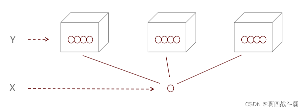
- All probability formula :
P(X) =P(Y1) x P(X | Y1) x P(Y2) x P(X | Y2) x…x P(Yn) x P(X | Yn) - Bayes theorem :
p ( Y = c k ∣ X = x ) = P ( X = x ∣ Y = c k ) P ( Y = c k ) ∑ k P ( X = x ∣ Y = c k ) P ( Y = c k ) p(Y=c_{k}|X=x)=\frac{P(X=x|Y=c_{k})P(Y=c_{k})}{\sum_{k}^{}P(X=x|Y=c_{k})P(Y=c_{k})} p(Y=ck∣X=x)=∑kP(X=x∣Y=ck)P(Y=ck)P(X=x∣Y=ck)P(Y=ck)
distinguish :
2、 Naive Bayesian theory
- Naive Bayesian method learns joint probability distribution through training data set P(X,Y), in other words , By learning class prior probability distribution and class conditional probability distribution .
- Naive Bayes method is used to calculate the conditional probability distribution Conditional independence Assumptions . Its name comes from Bayesian theorem and a simple assumption : The conditions of all features are independent of other given response variables , That is, the conditional independence assumption of characteristics .
Conditional independence hypothesis :
P ( X = x ∣ Y = c k ) = ∏ j = 1 n P ( X ( j ) = x ( j ) ∣ Y = c k ) P(X=x|Y=c_{k})=\prod_{j=1}^{n}P(X^{(j)}=x^{(j)}|Y=c_{k}) P(X=x∣Y=ck)=∏j=1nP(X(j)=x(j)∣Y=ck)
Naive Bayesian method actually learns the mechanism of generating data , So it belongs to generative . Conditional independence hypothesis means that the features used for classification are conditionally independent under the condition that the class is determined , This hypothesis makes the learning of naive Bayes possible .
Although this assumption makes the naive Bayesian method simple , But it will inevitably sacrifice a certain classification accuracy .
Naive Bayes classification , For the given input x, The learned model is used to calculate the posterior probability distribution P ( Y = c k ∣ X = x ) P(Y=c_{k}|X=x) P(Y=ck∣X=x), Take the class with the greatest posterior probability as x Class output of .
Naive Bayes classifier :
y = f ( x ) = a r g m a x P ( Y = c k ) ∏ j P ( X ( j ) = x ( j ) ∣ Y = c k ) ∑ k P ( Y = c k ) ∏ j P ( X ( j ) = x ( j ) ∣ Y = c k ) y=f(x)=argmax\frac{P(Y=c_{k})\prod_{j}^{}P(X^{(j)}=x^{(j)}|Y=c_{k})}{\sum_{k}^{}P(Y=c_{k})\prod_{j}^{}P(X^{(j)}=x^{(j)}|Y=c_{k})} y=f(x)=argmax∑kP(Y=ck)∏jP(X(j)=x(j)∣Y=ck)P(Y=ck)∏jP(X(j)=x(j)∣Y=ck)
Denominator to all c k c_{k} ck All the same :
y = a r g m a x P ( Y = c k ) ∏ j P ( X j = x j ∣ Y = c k ) y=arg maxP(Y=c_{k})\prod_{j}^{}P(X^{j}=x^{j}|Y=c_{k}) y=argmaxP(Y=ck)∏jP(Xj=xj∣Y=ck)
seek X Using the full probability formula , seek Y Using Bayesian theorem
The basic method of naive Bayes : On the basis of Statistics , According to conditional probability formula , Calculate the probability that the sample of the current feature belongs to a classification , Choose the largest probability Classification
This model is called naive because it assumes that all features are conditionally independent for response variables , But this assumption does not mean that all features are independent .
import numpy as np

X = np.array([[-1, -1], [-2, -1], [-3, -2], [1, 1], [2, 1], [3, 2]])
Y = np.array([1, 1, 1, 2, 2, 2])

from sklearn.naive_bayes import GaussianNB

clf = GaussianNB()

#  Fitting data
clf.fit(X, Y)
print("==[-0.8, -1] Predicted results ==")
print(clf.predict([[-0.8, -1]]))
print("==[3,2] Predicted results ==")
print(clf.predict([[3, 2]]))
3、 Bayesian decision theory and method
- In the classification problem , We will compare the data set characteristics of unknown tags with those of our known tags . Naive Bayes , It is such a method of comparison .
The basic idea :
- 1、 The parameter expression of conditional probability density and a priori probability are known
- 2、 Use Bayesian formula to convert to a posteriori probability
- 3、 Decision classification based on posterior probability
4、 Naive Bayesian classifier practice
simple ⻉ The most suitable scenario for Yess classification is text classification 、 Emotion analysis and spam identification . Among them, emotional analysis and garbage Email identification is through ⽂ Originally, I entered ⾏ Judge .
From here ⾥ You can see , These three scenarios are essentially text classification , this It is also simple ⻉ Ye Si is the best ⻓ Land ⽅. So simple ⻉ Ye Si often ⽤ On ⾃ But the language ⾔ Handle NLP Of ⼯ have .
sklearn Machine learning package sklearn The full name of Scikit-learn, It provides us with 3 A simple ⻉ Yess classification algorithm , Namely ⾼ Si Pu plain ⻉ Yess (GaussianNB)、 Polynomial simplicity ⻉ Yess (MultinomialNB) And Bernoulli are simple ⻉ Yess (BernoulliNB), The difference between them is the eigenvector x Distribution of .
According to the characteristic type of the algorithm, it is divided into two categories .
- continuity : This means that the final tag is a real value ( Decimals can exist )
- discrete : This means that the final result is the category value of the classification ( It can only be an integer )
5、 Bayesian classification algorithm
- Bayesian classification algorithm is a classification method based on Bayesian theorem and the assumption of feature condition independence .
These three algorithms are suitable for ⽤ In different scenarios , We should choose different algorithms according to different characteristic variables :
Gaussian naive Bayes
- Gaussian naive Bayes ( continuity ): Characteristic variables are continuous variables , In line with the Gaussian distribution
- for instance ⼈ The height of , The length of the object .

- for instance ⼈ The height of , The length of the object .
# Import the corresponding package
import numpy as np
# Import Gaussian model
from sklearn.naive_bayes import GaussianNB

# sample X It contains three features , Namely Red Percent of ,Green Percent of ,Blue Percent of
# The value of each characteristic is (0,1) Decimal between

# First, we create a training set
X = np.array([[0.5, 0, 0.5], [1, 1, 0], [0, 0, 0]])
# Given the classification label of our training set
y = np.array(['Purple', 'Yellow', 'Black'])

# Use Gaussian model to train data
clf = GaussianNB()
# Training data set
clf.fit(X, y)

# Now we use our model to test
# For example, let's try ,red 0.5,green 0.5,blue 0.5
print(clf.predict([[0.5, 0.5, 0.5]]))
Polynomial naive Bayes
- Polynomial naive Bayes ( discrete ): Characteristic variables are discrete variables , According to the multinomial distribution , When the features are classified , Polynomial models can be used . Multinomial distribution describes the probability distribution in the sample label .
- It can be used to calculate the occurrence frequency of classification in features . In particular , When there are only two characteristics , Bernoulli model in polynomial model will be used .
- In document classification, feature variables are reflected in ⼀ The number of times a word appears
- Or words TF-IDF It's worth waiting for .
# Import related packages
import numpy as np
# Import polynomial model
from sklearn.naive_bayes import MultinomialNB

# We use the data set of fruit at the beginning of the article as an example
# Samples of the fruit dataset X It has three characteristics [Size, Weight, Color]
# There are three categories for each feature
# because python Unable to recognize characters directly
# Therefore, the different classifications of these three features are recoded as follows
# Size: 0 = Small, 1 = Moderate, 2 = Large
# Weight: 0 = Light, 1 = Moderate, 2 = Heavy
# Color: 0 = Red, 1 = Blue, 2 = Brown

# Create a training set with encoded data
X = np.array([[1, 1, 0], [0, 0, 1], [2, 2, 2]])
# Create labels for the data of the training set
y = np.array(['Apple', 'Blueberry', 'Coconut'])

# Use polynomial model to train data
clf = MultinomialNB()
# Training fruit data set
clf.fit(X, y)

# Forecast data set
# For example, let's try  size = 1,weight = 2,color = 0
print(clf.predict([[1, 2, 0]]))
Bernoulli naive Bayes
- Bernoulli naive Bayes ( discrete ): Characteristic variables are Boolean variables , accord with 0/1 Distribution , Generally speaking, it is a two category label . As mentioned above , When there are only two characteristics , We can use Bernoulli model .
- Different from polynomial model , Here we only calculate whether one feature occurs .
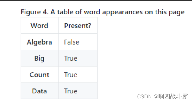
- such as , Does this page exist 【 polynomial 】 These three words , There are only two answers , There is or non-existent .
- The calculation method of conditional probability of Bernoulli model is consistent with polynomial model . In document classification, the feature is whether words appear .
# Import package
import numpy as np
# Import Bernoulli model
from sklearn.naive_bayes import BernoulliNB

# Data sets X There are three characteristics of , Namely
# Walks like a duck
# Talks like a duck
# Is small]
# These three characteristics have two distributions , yes or no
# Walks like a duck: 0 = False, 1 = True
# Talks like a duck: 0 = False, 1 = True
# Is small: 0 = False, 1 = True

# Create training set
X = np.array([[1, 1, 0], [0, 0, 1], [1, 0, 0]])
# Create labels for training sets
# It's a duck or Not a duck
y = np.array(['Duck', 'Not a Duck', 'Not a Duck'])

# Use Bernoulli model to train data
clf = BernoulliNB()
# Training data set
clf.fit(X, y)

# Forecast data set
# For example, let's try   The three characteristics are true When , Is it a duck
print( clf.predict([[1, 1, 1]]))
边栏推荐
- Microservice practice | load balancing component and source code analysis
- Chrome浏览器标签管理插件–OneTab
- C# 百度地图,高德地图,Google地图(GPS) 经纬度转换
- Function ‘ngram‘ is not defined
- The channel cannot be viewed when the queue manager is running
- C language - Blue Bridge Cup - 7 segment code
- 微服务实战|微服务网关Zuul入门与实战
- AMQ 4043 solution for errors when using IBM MQ remote connection
- QT -- how to set shadow effect in QWidget
- WSL installation, beautification, network agent and remote development
猜你喜欢

【Go实战基础】gin 如何验证请求参数

【Go实战基础】gin 如何设置路由
Matplotlib剑客行——没有工具用代码也能画图的造型师
汉诺塔问题的求解与分析

I've taken it. MySQL table 500W rows, but someone doesn't partition it?

Cloud computing in my eyes - PAAS (platform as a service)

Mysql安装时mysqld.exe报`应用程序无法正常启动(0xc000007b)`
Chrome浏览器标签管理插件–OneTab
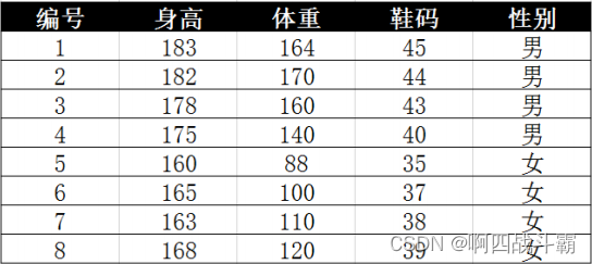
Data type case of machine learning -- using data to distinguish men and women based on Naive Bayesian method

Chrome用户脚本管理器-Tampermonkey 油猴
随机推荐
Microservice practice | load balancing component and source code analysis
统计字符串中各类字符的个数
ORA-12514问题解决方法
[go practical basis] how to set the route in gin
Watermelon book -- Chapter 5 neural network
[staff] common symbols of staff (Hualian clef | treble clef | bass clef | rest | bar line)
Flink-使用流批一体API统计单词数量
微服务实战|声明式服务调用OpenFeign实践
汉诺塔问题的求解与分析
Multi version concurrency control mvcc of MySQL
机器学习实战:《美人鱼》属于爱情片还是动作片?KNN揭晓答案
C# 调用系统声音 嘀~
Installing Oracle database 19C RAC on Linux
Select sort and insert sort
Openshift container platform community okd 4.10.0 deployment
oracle删除表空间及用户
Gocv image cutting and display
How to realize asynchronous programming in a synchronous way?
A detailed explanation takes you to reproduce the statistical learning method again -- Chapter 2, perceptron model
机器学习之数据类型案例——基于朴素贝叶斯法,用数据辩男女