当前位置:网站首页>Machine learning summary (I): linear regression, ridge regression, Lasso regression
Machine learning summary (I): linear regression, ridge regression, Lasso regression
2022-07-01 13:33:00 【Full stack programmer webmaster】
Hello everyone , I meet you again , I'm your friend, Quan Jun .
Linear regression as a regression analysis technology , The dependent variable of its analysis belongs to continuous variable , If the dependent variable is transformed into a discrete variable , Turn it into a classification problem . Regression analysis belongs to supervised Study problem , This blog will focus on reviewing the knowledge points of standard linear regression , And the possible problems in linear regression are briefly discussed , Two variants of linear regression, ridge regression and Lasso Return to , Finally through sklearn The library simulates the whole regression process .
Directory structure
- General form of linear regression
- Possible problems in linear regression
- Over fitting problem and its solution
- Linear regression code implementation
- The return of the mountains and the future Lasso Return to
- Ridge regression and Lasso Regression code implementation
General form of linear regression
Possible problems in linear regression
- There are two ways to solve the minimum value of the loss function : Gradient descent method and normal equation , The comparison between the two is listed in the attached notes .
- Feature scaling : That is to normalize the characteristic data , There are two benefits of feature scaling , First, it can improve the convergence speed of the model , Because if the data difference between features is large , Take two characteristics , Take these two features as horizontal and vertical coordinates to draw contour map , Drawn is a flat ellipse , At this time, finding the gradient direction through the gradient descent method will eventually take a zigzag route perpendicular to the contour , The iteration speed becomes slower . But if the feature is normalized , The entire contour map will appear circular , The direction of the gradient points to the center of the circle , The iteration speed is much faster than the former . Second, it can improve the accuracy of the model .
- Learning rate α Selection of : If learning rate α Selection too small , It will lead to more iterations , The convergence rate slows down ; Learning rate α The selection is too large , It is possible to skip the optimal solution , Eventually, there is no convergence at all .
Over fitting problem and its solution
- problem : The following picture shows the fitting problem
- resolvent :(1): Discard some features that have little impact on our final prediction , Specific features that need to be discarded can be passed PCA Algorithm to achieve ;(2): Using regularization techniques , Keep all features , But reduce the parameters in front of the feature θ Size , Specifically, you can modify the form of loss function in linear regression , Ridge regression and Lasso This is what regression does .
Linear regression code example
import matplotlib.pyplot as plt
import numpy as np
from sklearn import datasets, linear_model, discriminant_analysis, cross_validation

def load_data():
    diabetes = datasets.load_diabetes()
    return cross_validation.train_test_split(diabetes.data, diabetes.target, test_size=0.25, random_state=0)

def test_LinearRegression(*data):
    X_train, X_test, y_train, y_test = data
    # adopt sklearn Of linear_model Create a linear regression object
    linearRegression = linear_model.LinearRegression()
    # Training
    linearRegression.fit(X_train, y_train)
    # adopt LinearRegression Of coef_ Attribute gets the weight vector ,intercept_ get b Value
    print(" The weight vector :%s, b The value of is :%.2f" % (linearRegression.coef_, linearRegression.intercept_))
    # Calculate the value of the loss function
    print(" The value of the loss function : %.2f" % np.mean((linearRegression.predict(X_test) - y_test) ** 2))
    # Calculate the predicted performance score
    print(" Predict performance scores : %.2f" % linearRegression.score(X_test, y_test))

if __name__ == '__main__':
    # Acquired data set
    X_train, X_test, y_train, y_test = load_data()
    # Perform training and output prediction results
test_LinearRegression(X_train, X_test, y_train, y_test)Linear regression example output
 The weight vector :[ -43.26774487 -208.67053951  593.39797213  302.89814903 -560.27689824
  261.47657106   -8.83343952  135.93715156  703.22658427   28.34844354], b The value of is :153.07
 The value of the loss function : 3180.20
Predict performance scores : 0.36The return of the mountains and the future Lasso Return to
The return of the mountains and the future Lasso The emergence of regression is to solve the over fitting of linear regression and solve it by normal equation method θ In the process of x Transpose times x The problem of irreversibility , These two kinds of regression achieve their goals by introducing regularization terms into the loss function , See the following figure for the comparison of the loss functions of the three :
among λ It is called regularization parameter , If λ The selection is too large , Will put all the parameters θ Minimize , Cause under fitting , If λ Selection too small , It will cause the over fitting problem to be solved improperly , therefore λ The selection of is a technical activity . The return of the mountains and the future Lasso The biggest difference of regression is that ridge regression introduces L2 Norm penalty term ,Lasso Regression introduces L1 Norm penalty term ,Lasso Regression can make many of the loss functions θ All become 0, This is better than ridge regression , Because the return of the ridge requires all θ All exist , In this way, the amount of calculation Lasso The return will be much smaller than the ridge return .
You can see ,Lasso The regression will eventually tend to a straight line , The reason is that there are many θ The values have all been 0, The ridge regression has a certain smoothness , Because of all the θ All values exist .
Ridge regression and Lasso Regression code implementation
Ridge regression code example
import matplotlib.pyplot as plt
import numpy as np
from sklearn import datasets, linear_model, discriminant_analysis, cross_validation

def load_data():
    diabetes = datasets.load_diabetes()
    return cross_validation.train_test_split(diabetes.data, diabetes.target, test_size=0.25, random_state=0)

def test_ridge(*data):
    X_train, X_test, y_train, y_test = data
    ridgeRegression = linear_model.Ridge()
    ridgeRegression.fit(X_train, y_train)
    print(" The weight vector :%s, b The value of is :%.2f" % (ridgeRegression.coef_, ridgeRegression.intercept_))
    print(" The value of the loss function :%.2f" % np.mean((ridgeRegression.predict(X_test) - y_test) ** 2))
    print(" Predict performance scores : %.2f" % ridgeRegression.score(X_test, y_test))

# Test different α Effect of value on prediction performance
def test_ridge_alpha(*data):
    X_train, X_test, y_train, y_test = data
    alphas = [0.01, 0.02, 0.05, 0.1, 0.2, 0.5, 1, 2, 5, 10, 20, 50, 100, 200, 500, 1000]
    scores = []
    for i, alpha in enumerate(alphas):
        ridgeRegression = linear_model.Ridge(alpha=alpha)
        ridgeRegression.fit(X_train, y_train)
        scores.append(ridgeRegression.score(X_test, y_test))
    return alphas, scores

def show_plot(alphas, scores):
    figure = plt.figure()
    ax = figure.add_subplot(1, 1, 1)
    ax.plot(alphas, scores)
    ax.set_xlabel(r"$\alpha$")
    ax.set_ylabel(r"score")
    ax.set_xscale("log")
    ax.set_title("Ridge")
    plt.show()

if __name__ == '__main__':
    # Use default alpha
    # Acquired data set
    #X_train, X_test, y_train, y_test = load_data()
    # Train and predict the results
    #test_ridge(X_train, X_test, y_train, y_test)

    # Use your own alpha
    X_train, X_test, y_train, y_test = load_data()
    alphas, scores = test_ridge_alpha(X_train, X_test, y_train, y_test)
show_plot(alphas, scores)Lasso Regression code example
import matplotlib.pyplot as plt
import numpy as np
from sklearn import datasets, linear_model, discriminant_analysis, cross_validation

def load_data():
    diabetes = datasets.load_diabetes()
    return cross_validation.train_test_split(diabetes.data, diabetes.target, test_size=0.25, random_state=0)

def test_lasso(*data):
    X_train, X_test, y_train, y_test = data
    lassoRegression = linear_model.Lasso()
    lassoRegression.fit(X_train, y_train)
    print(" The weight vector :%s, b The value of is :%.2f" % (lassoRegression.coef_, lassoRegression.intercept_))
    print(" The value of the loss function :%.2f" % np.mean((lassoRegression.predict(X_test) - y_test) ** 2))
    print(" Predict performance scores : %.2f" % lassoRegression.score(X_test, y_test))

# Test different α Effect of value on prediction performance
def test_lasso_alpha(*data):
    X_train, X_test, y_train, y_test = data
    alphas = [0.01, 0.02, 0.05, 0.1, 0.2, 0.5, 1, 2, 5, 10, 20, 50, 100, 200, 500, 1000]
    scores = []
    for i, alpha in enumerate(alphas):
        lassoRegression = linear_model.Lasso(alpha=alpha)
        lassoRegression.fit(X_train, y_train)
        scores.append(lassoRegression.score(X_test, y_test))
    return alphas, scores

def show_plot(alphas, scores):
    figure = plt.figure()
    ax = figure.add_subplot(1, 1, 1)
    ax.plot(alphas, scores)
    ax.set_xlabel(r"$\alpha$")
    ax.set_ylabel(r"score")
    ax.set_xscale("log")
    ax.set_title("Ridge")
    plt.show()

if __name__=='__main__':
    X_train, X_test, y_train, y_test = load_data()
    #  Use default alpha
    #test_lasso(X_train, X_test, y_train, y_test)
    #  Use your own alpha
    alphas, scores = test_lasso_alpha(X_train, X_test, y_train, y_test)
show_plot(alphas, scores)Attach study notes
reference
- python War machine learning
- Andrew Ng Machine learning open class
- http://www.jianshu.com/p/35e67c9e4cbf
- http://freemind.pluskid.org/machine-learning/sparsity-and-some-basics-of-l1-regularization/#ed61992b37932e208ae114be75e42a3e6dc34cb3
Publisher : Full stack programmer stack length , Reprint please indicate the source :https://javaforall.cn/131445.html Link to the original text :https://javaforall.cn
边栏推荐
- 【大型电商项目开发】性能压测-压力测试基本概念&JMeter-38
- Cs5268 advantages replace ag9321mcq typec multi in one docking station scheme
- In the next stage of digital transformation, digital twin manufacturer Youyi technology announced that it had completed a financing of more than 300 million yuan
- 受益互联网出海 汇量科技业绩重回高增长
- 7. Icons
- Report on the 14th five year plan and future development trend of China's integrated circuit packaging industry Ⓓ 2022 ~ 2028
- Who should I know when opening a stock account? Is it actually safe to open an account online?
- PG basics -- Logical Structure Management (trigger)
- What is the future development direction of people with ordinary education, appearance and family background? The career planning after 00 has been made clear
- Spark source code (V) how does dagscheduler taskscheduler cooperate with submitting tasks, and what is the corresponding relationship between application, job, stage, taskset, and task?
猜你喜欢

北斗通信模块 北斗gps模块 北斗通信终端DTU

The stack size specified is too small, specify at least 328k

What is the future development direction of people with ordinary education, appearance and family background? The career planning after 00 has been made clear
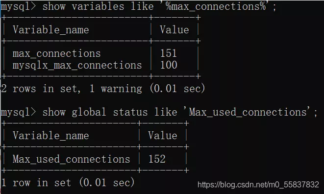
Reasons for MySQL reporting 1040too many connections and Solutions

Content Audit Technology

minimum spanning tree

Jenkins+webhooks-多分支参数化构建-

刘对(火线安全)-多云环境的风险发现

进入前六!博云在中国云管理软件市场销量排行持续上升

Colorful five pointed star SVG dynamic web page background JS special effect
随机推荐
Explain IO multiplexing, select, poll, epoll in detail
9. Use of better scroll and ref
ZABBIX 6.0 source code installation and ha configuration
During Oracle CDC data transmission, the CLOB type field will lose its value during update. There is a value before update, but
SAP 智能机器人流程自动化(iRPA)解决方案分享
声明一个抽象类Vehicle,它包含私有变量numOfWheels和公共函数Vehicle(int)、Horn()、setNumOfWheels(int)和getNumOfWheels()。子类Mot
Three questions about scientific entrepreneurship: timing, pain points and important decisions
Report on the 14th five year plan and future development trend of China's integrated circuit packaging industry Ⓓ 2022 ~ 2028
面试题目总结(1) https中间人攻击,ConcurrentHashMap的原理 ,serialVersionUID常量,redis单线程,
1553B environment construction
Yarn restart applications record recovery
Detailed explanation of parallel replication examples in MySQL replication
孔松(信通院)-数字化时代云安全能力建设及趋势
How much money do novices prepare to play futures? Is agricultural products OK?
Yarn重启applications记录恢复
The future of game guild in decentralized games
波浪动画彩色五角星loader加载js特效
开源者的自我修养|为 ShardingSphere 贡献了千万行代码的程序员,后来当了 CEO
Research Report on China's software outsourcing industry investment strategy and the 14th five year plan Ⓡ 2022 ~ 2028
科学创业三问:关于时机、痛点与重要决策