Decision tree algorithm theory

WeChat official account ： Manon charging station pro
Personal home page ：https://codeshellme.github.io

1, What is a decision tree ？

Decision tree is a machine learning algorithm , We can use decision trees to deal with classification problems . Decision tree decision making （ classification ） The process can be expressed in an inverted tree structure , So it's called decision tree .

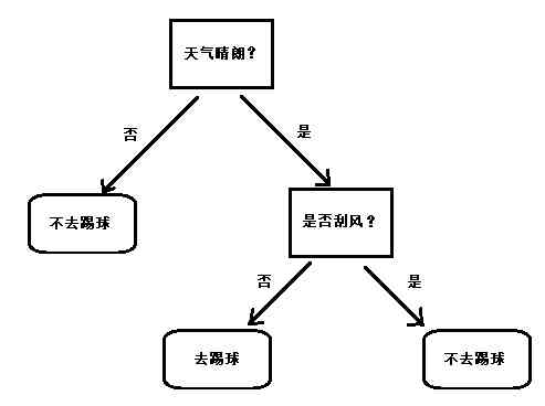
For example, we depend on the weather Whether it's sunny or not and Is it windy To decide whether to play football or not ？ When it's sunny and windless , We just went to play football .

here , The decision process can be represented in a tree structure , as follows ：

---

---

This is the simplest decision tree , We can use it to judge whether we want to play football . At the top is the root node of the tree , At the bottom is the leaf node of the tree . In the box is the process of judgment , In the oval is the result of the decision .

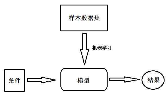
Of course , In actual use , The judgment condition is not so simple , And we won't let us draw our own pictures by hand . Practical application , We'll make the program automatic , This decision tree is constructed from a set of sample data , This program automatically builds the decision tree process is machine learning The process of .

The final decision tree is the result of machine learning , be called Model . Last , We can put some... Into the model Property conditions , Let the model give us Judge the result .

---

---

2, How to build a decision tree ？

For example, we have the following data sets ：

Serial number	Conditions : It's sunny ?	Conditions : Is it windy ?	result : To play football ?
1	yes	no	Go to
2	yes	yes	Don't go to
3	no	yes	Don't go to
4	no	no	Don't go to

You can see in this table that 4 That's ok （ The first row header doesn't count ）,4 Column data .

Generally in machine learning , The last column is called The goal is (target), The first column is called features (features).

We're going to use this data set , To build a decision tree , So how to build ？

First , You need to determine which attribute to use as the first criterion , It's to judge first It's sunny , Or judge first Is it windy ？ That is to say , Let the weather be the root node of the tree , Or let the wind be the root node of the tree ？

To solve this problem, we need to use Information entropy and Information purity The concept of , Let's first look at what information entropy is .

3, What is information entropy ？

1948 year , Claude · Xiangnong is in his paper “ The mathematical principle of communication ” Mentioned in the Information entropy （ It's usually used H Express ）, The unit for measuring information entropy is The bit .

That is to say , The amount of information can be quantified . The amount of information in a piece is related to the uncertainty of information , It can be said that , The amount of information is equal to the amount of uncertainty （ The uncertainty of information ）.

The formula of information entropy is as follows ：

---

---

The meaning of the formula is ：

• Things to be classified can be divided into several categories , there n It's the number of categories .
• H(X) It's entropy , The mathematical meaning is , All categories contain information expectations .
• -㏒p(Xì) Represents the information value of the symbol ,p(Xì) Is the probability of choosing the classification .
• Formula log General with 2 Bottom .

All in all , Just to know , The amount of information can be calculated by mathematical formula , In terms of information theory, it's called information entropy . The greater the entropy of information , The more information there is .

3.1, Calculate entropy of information

So let's calculate the information entropy of the above table data . We only focus on “ result ” That column ：

result : To play football ?

Go to

Don't go to

Don't go to

Don't go to

According to the form , We can know , All categories share 2 Kind of , That is to say “ Go to ” and “ Don't go to ”,“ Go to ” There is 1 Time ,“ Don't go to ” There is 3 Time .

Separate calculation “ Go to ” and “ Don't go to ” Probability of occurrence ：

• P( Go to ) = 1 / 4 = 0.25
• P( Don't go to ) = 3 / 4 = 0.75

then , Calculate according to the formula of entropy “ Go to ” and “ Don't go to ” The entropy of information , among log With 2 Bottom ：

• H( Go to ) = 0.25 * log 0.25 = -0.5
• H( Don't go to ) = 0.74 * log 0.75 = -0.31127812445913283

therefore , The amount of information contained in the whole table is ：

• H( form ) = -(H( Go to ) + H( Don't go to )) = 0.81127812445913283

3.2, Using code to realize the calculation of information entropy

The process of calculating information entropy is used Python Code implementation , as follows ：

import math

#  This function is used to calculate the information entropy of a set of data 
# data_set  It's a list , Represents a set of data 
# data_set  The elements of data  It's also a list 
def calc_ent(data_set):
    labels = {} #  Used to count each label  The number of 
    
    for data in data_set:
        label = data[-1]	#  Only the last element is used for calculation 
        if label not in labels:
            labels[label] = 0

        labels[label] += 1 

    ent = 0 #  entropy 
    n = len(data_set)   #  Number of data 

    #  Calculate entropy of information 
    for label in labels:
        prob = float(labels[label]) / n # label  Probability 
        ent -= prob * math.log(prob, 2) #  According to the formula of information entropy 

    return ent

This function is used to calculate the information entropy of the table ：

#  Convert the table to  python  list 
# "yes"  Express " Go to "
# "no"  Express " Don't go to "
data_set = [['yes'], ['no'], ['no'], ['no']] 
ent = calc_ent(data_set)
print(ent)	# 0.811278124459

so , The result of code calculation is 0.811278124459, With the result of our manual calculation 0.81127812445913283 It's the same （ The number of decimal places reserved is different ）.

4, What is information purity ？

The purity of information is inversely proportional to information entropy ：

• The greater the entropy of information , The more information , The more messy the information is , The lower the purity .
• The less entropy of information , The less information , The more regular the information is , The higher the purity .

classical “ Impure ” There are three algorithms , Namely ：

• Information gain , namely ID3 Algorithm ,Information Divergence, The algorithm consists of Ross Quinlan On 1975 in , Can be used to generate a binary tree or a multi tree .
  • ID3 The algorithm will select the attribute with the largest information gain as the partition of attributes .
• Information gain rate , namely C4.5 Algorithm , yes Ross Quinlan stay ID3 Based on the improved algorithm , Can be used to generate a binary tree or a multi tree .
• Gini is not pure , namely CART Algorithm ,Classification and Regression Trees, Chinese is Categorizing regression trees .
  • It can be used for classification number , It can also be used for regression trees . Classification trees use The gini coefficient Do judgment , Return to the tree with deviation Do judgment .
  • The Gini coefficient itself reflects the uncertainty of the sample .
    • When the Gini coefficient is smaller , The smaller the difference between the samples , The less uncertainty .
    • CART Algorithm The attribute with the smallest Gini coefficient will be selected as the attribute partition .

Information gain is one of the simplest algorithms , The latter two are derived from it . In this article , We're just going to go into details about information gain .

The gini coefficient It is a common indicator used to measure the income gap of a country in economics . When the Gini coefficient is greater than 0.4 When , It shows that there are great differences in wealth . The Gini coefficient is in 0.2-0.4 The distribution is reasonable , The wealth gap is not big .

5, What is information gain ？

Information gain is , Before and after partitioning a dataset according to a property , Changes in the amount of information .

The formula of information gain is as follows ：

The meaning of the formula ：

• In short ：G = H( Parent node ) - H( All child nodes )
• That is to say ： The information entropy of the parent node subtracts the information entropy of all the child nodes .
• The information entropy of all the child nodes will be calculated according to the probability of the child node appearing in the parent node , It's called Normalized information entropy .

The purpose of information gain is , The purity improvement after partitioning the data set , That is, the decrease of information entropy . If the data set is divided according to a certain attribute , Can obtain the maximum information gain , So this property is the best choice .

therefore , We want to find the root node , We need to calculate the information gain of each attribute as the root node , Then get the attribute with the most information gain , It's the root node .

5.1, Calculated information gain

For the sake of convenience , I put the form above here ：

Serial number	Conditions : It's sunny ?	Conditions : Is it windy ?	result : To play football ?
1	yes	no	Go to
2	yes	yes	Don't go to
3	no	yes	Don't go to
4	no	no	Don't go to

We already know that , Information gain is equal to the difference of information entropy before and after dividing according to a certain attribute .

We already know the entropy of information before this table is partitioned , That's what we calculated above ：

• H( form ) = 0.81127812445913283.

Next , We calculate according to “ It's sunny ” Divided information gain . according to “ It's sunny ” After dividing, there are two tables .

form 1,“ It's sunny ” The value of is “ yes ”：

Serial number	Conditions : It's sunny ?	Conditions : Is it windy ?	result : To play football ?
1	yes	no	Go to
2	yes	yes	Don't go to

Classification has something in common 2 Kind of , That is to say “ Go to ” and “ Don't go to ”,“ Go to ” There is 1 Time ,“ Don't go to ” There is 1 Time .

therefore ,“ Go to ” and “ Don't go to ” The probability of occurrence is 0.5：

• P( Go to ) = P( Don't go to ) = 1 / 2 = 0.5

then ,“ Go to ” and “ Don't go to ” The entropy of information , among log With 2 Bottom ：

• H( Go to ) = H( Don't go to ) = 0.5 * log 0.5 = -0.5

therefore , form 1 The amount of information contained is ：

• H( form 1) = -(H( Go to ) + H( Don't go to )) = 1

form 2,“ It's sunny ” The value of is “ no ”：

Serial number	Conditions : It's sunny ?	Conditions : Is it windy ?	result : To play football ?
3	no	yes	Don't go to
4	no	no	Don't go to

All the classifications are only 1 Kind of , yes “ Don't go to ”. therefore ：

• P( Don't go to ) = 1

then ,“ Don't go to ” The entropy of information , among log With 2 Bottom ：

• H( Don't go to ) = 1 * log 1 = 0

therefore , form 2 The amount of information contained is ：

• H( form 2) = 0

The total data share 4 Share ：

• form 1 There is 2 Share , The probability of 2/4 = 0.5
• form 2 There is 2 Share , The probability of 2/4 = 0.5

therefore , Finally according to “ It's sunny ” The information gain of the partition is ：

• G( It's sunny ) = H( form ) - (0.5*H( form 1) + 0.5*H( form 2)) = H( form ) - 0.5 = 0.31127812445913283.

5.2,ID3 Disadvantages of the algorithm

When we calculate more information gain , You'll find that ,ID3 The algorithm tends to select the attribute with more values as （ root ） node .

But sometimes , Some properties don't affect the result （ Or it has little effect on the results ）, Then use ID3 The selected attributes are not appropriate .

To improve ID3 This shortcoming of the algorithm ,C4.5 The algorithm came into being .

C4.5 Algorithm to ID3 The improvements of the algorithm include ：

• Using information gain rate , It's not information gain , avoid ID3 The algorithm tends to choose the attribute with more values .
• Added pruning technology , prevent ID3 The occurrence of over fitting in the algorithm .
• Discretization of continuous attributes , bring C4.5 The algorithm can handle the case of continuous attributes , and ID3 Can only handle discrete data .
• Handling missing values ,C4.5 It can also deal with incomplete data sets .

Of course C4.5 The algorithm is not without shortcomings , because C4.5 The algorithm needs to scan the data set many times , So the efficiency of the algorithm is relatively low . There's no more discussion here C4.5 Algorithm .

The next part will introduce how to use decision tree to solve practical problems .

---

Welcome to follow the author's official account , Get more technical dry goods .