当前位置:网站首页>[deep learning] image hyperspectral experiment: srcnn/fsrcnn
[deep learning] image hyperspectral experiment: srcnn/fsrcnn
2022-07-07 15:07:00 【zstar-_】
Image super-resolution is super-resolution , Change the image from blurred to clear
This paper is the experimental report of deep learning professional courses , Complete source code file / See the end of the text for the data set acquisition method
1. The goal of the experiment
The input size is h×w Image X, Output as a sh×sw Image Y,s Is the magnification .
2. Data set profile
This experiment uses BSDS500 Data sets , The training set contains 200 Zhang image , The validation set contains 100 Zhang image , The test set contains 200 Zhang image .
Data set source :https://download.csdn.net/download/weixin_42028424/11045313
3. Data preprocessing
Data preprocessing consists of two steps :
(1) Convert picture to YCbCr Pattern
because RGB Color mode hue 、 chroma 、 Saturation is difficult to separate when the three are mixed together , So convert it into YcbCr Color mode ,Y Is the luminance component ,Cb Express RGB The blue part of the input signal and RGB The difference between signal brightness values ,Cr Express RGB The red part of the input signal and RGB The difference between signal brightness values .
(2) Cut the picture into 300×300 The square of
Because the neural network input image used later requires the same length and width , and BSDS500 The length and width of the pictures in the dataset are not consistent , Therefore, it needs to be cut . The method used here is to locate the center of each picture first , Then take the center of the picture as the benchmark , Expand in four directions 150 Pixel , To crop the picture into 300×300 The square of .
Related codes :
def is_image_file(filename):
    return any(filename.endswith(extension) for extension in [".png", ".jpg", ".jpeg"])


def load_img(filepath):
    img = Image.open(filepath).convert('YCbCr')
    y, _, _ = img.split()
    return y


CROP_SIZE = 300


class DatasetFromFolder(Dataset):
    def __init__(self, image_dir, zoom_factor):
        super(DatasetFromFolder, self).__init__()
        self.image_filenames = [join(image_dir, x)
                                for x in listdir(image_dir) if is_image_file(x)]
        crop_size = CROP_SIZE - (CROP_SIZE % zoom_factor)
        #  Cut from the center of the picture into 300*300
        self.input_transform = transforms.Compose([transforms.CenterCrop(crop_size),
                                                   transforms.Resize(
                                                       crop_size // zoom_factor),
                                                   transforms.Resize(
                                                       crop_size, interpolation=Image.BICUBIC),
                                                   # BICUBIC  Bicubic interpolation
                                                   transforms.ToTensor()])
        self.target_transform = transforms.Compose(
            [transforms.CenterCrop(crop_size), transforms.ToTensor()])

    def __getitem__(self, index):
        input = load_img(self.image_filenames[index])
        target = input.copy()
        input = self.input_transform(input)
        target = self.target_transform(target)
        return input, target

    def __len__(self):
        return len(self.image_filenames)
4. Network structure
This experiment tried SRCNN and FSRCNN Two networks .
4.1 SRCNN
SRCNN from 2014 year Chao Dong And so on , It is the first work of deep learning in the field of image hypersegmentation . The network structure is shown in the figure below :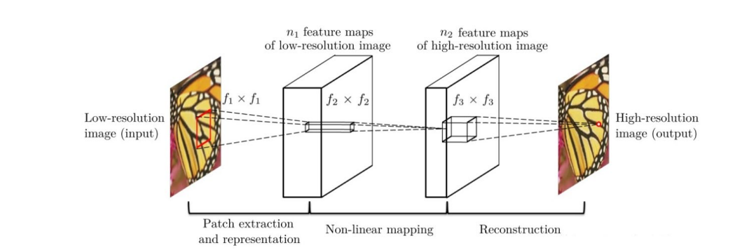
The network for a low resolution image , First, use bicubic interpolation to enlarge it to the target size , Then do nonlinear mapping through three-layer convolution network , The result obtained is output as a high-resolution image .
The author's explanation of the three convolution layers :
(1) Feature block extraction and representation : This operation starts from a low resolution image Y Extract overlapping feature blocks , Each feature block is represented as a high-dimensional vector . These vectors consist of a set of characteristic graphs , Its number is equal to the dimension of the vector .
(2) Nonlinear mapping : This operation nonlinearly maps each high-dimensional vector to another high-dimensional vector . Each mapping vector is conceptually the representation of high-resolution feature blocks . These vectors also include another set of characteristic graphs .
(3) The reconstruction : This operation aggregates the above high resolution patch-wise( An area between the pixel level and the image level ) Express , Generate the final high resolution image .
Each layer structure :
- Input : Processed low resolution image
- Convolution layer 1: use 9×9 Convolution kernel
- Convolution layer 2: use 1×1 Convolution kernel
- Convolution layer 3: use 5×5 Convolution kernel
- Output : High resolution image
Model structure code :
class SRCNN(nn.Module):
    def __init__(self, upscale_factor):
        super(SRCNN, self).__init__()

        self.relu = nn.ReLU()
        self.conv1 = nn.Conv2d(1, 64, kernel_size=5, stride=1, padding=2)
        self.conv2 = nn.Conv2d(64, 64, kernel_size=3, stride=1, padding=1)
        self.conv3 = nn.Conv2d(64, 32, kernel_size=3, stride=1, padding=1)
        self.conv4 = nn.Conv2d(32, upscale_factor ** 2,
                               kernel_size=3, stride=1, padding=1)
        self.pixel_shuffle = nn.PixelShuffle(upscale_factor)

        self._initialize_weights()

    def _initialize_weights(self):
        init.orthogonal_(self.conv1.weight, init.calculate_gain('relu'))
        init.orthogonal_(self.conv2.weight, init.calculate_gain('relu'))
        init.orthogonal_(self.conv3.weight, init.calculate_gain('relu'))
        init.orthogonal_(self.conv4.weight)

    def forward(self, x):
        x = self.conv1(x)
        x = self.relu(x)
        x = self.conv2(x)
        x = self.relu(x)
        x = self.conv3(x)
        x = self.relu(x)
        x = self.conv4(x)
        x = self.pixel_shuffle(x)
        return x
4.2 FSRCNN
FSRCNN from 2016 year Chao Dong And so on , And SRCNN Is the same author . The network structure is shown in the figure below :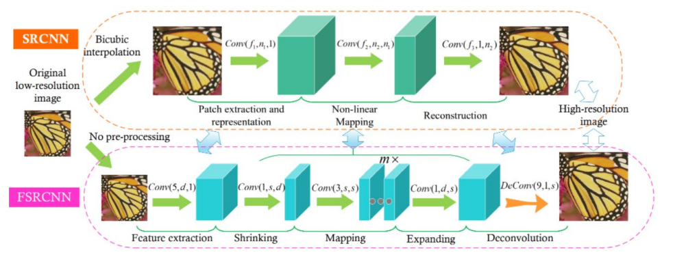
FSRCNN stay SRCNN On this basis, the following changes have been made :
1.FSRCNN The low resolution image is directly used as the input , differ SRCNN The low resolution image needs to be interpolated by bicubic interpolation first, and then used as input ;
2.FSRCNN At the end of the network, the deconvolution layer is used to realize up sampling ;
3.FSRCNN There is no nonlinear mapping in , There is a corresponding contraction 、 Mapping and extension ;
4.FSRCNN Choose smaller filters and deeper network structures .
Each layer structure :
- Input layer :FSRCNN Don't use bicubic Interpolation to upsample the input image , It goes directly into the feature extraction layer
- Feature extraction layer : use 1 × d × ( 5 × 5 ) Convolution layer extraction
- Shrinkage layer : use d × s × ( 1 × 1 ) Convolution layer to reduce the number of channels , To reduce the complexity of the model
- Mapping layer : use s × s × ( 3 × 3 ) The convolution layer is used to increase the nonlinearity of the model LR → SR Mapping
- Expansion layer : The layer and the shrinkage layer are symmetrical , use s × d × ( 1 × 1 ) Convolution layer to increase the expressiveness of reconstruction
- Deconvolution layer :s × 1 × ( 9 × 9 )
- Output layer : Output HR Images
Model structure code :
class FSRCNN(nn.Module):
    def __init__(self, scale_factor, num_channels=1, d=56, s=12, m=4):
        super(FSRCNN, self).__init__()
        self.first_part = nn.Sequential(
            nn.Conv2d(num_channels, d, kernel_size=5, padding=5//2),
            nn.PReLU(d)
        )
        self.mid_part = [nn.Conv2d(d, s, kernel_size=1), nn.PReLU(s)]
        for _ in range(m):
            self.mid_part.extend([nn.Conv2d(s, s, kernel_size=3, padding=3//2), nn.PReLU(s)])
        self.mid_part.extend([nn.Conv2d(s, d, kernel_size=1), nn.PReLU(d)])
        self.mid_part = nn.Sequential(*self.mid_part)
        self.last_part = nn.ConvTranspose2d(d, num_channels, kernel_size=9, stride=scale_factor, padding=9//2,
                                            output_padding=scale_factor-1)

        self._initialize_weights()

    def _initialize_weights(self):
        for m in self.first_part:
            if isinstance(m, nn.Conv2d):
                nn.init.normal_(m.weight.data, mean=0.0, std=math.sqrt(2/(m.out_channels*m.weight.data[0][0].numel())))
                nn.init.zeros_(m.bias.data)
        for m in self.mid_part:
            if isinstance(m, nn.Conv2d):
                nn.init.normal_(m.weight.data, mean=0.0, std=math.sqrt(2/(m.out_channels*m.weight.data[0][0].numel())))
                nn.init.zeros_(m.bias.data)
        nn.init.normal_(self.last_part.weight.data, mean=0.0, std=0.001)
        nn.init.zeros_(self.last_part.bias.data)

    def forward(self, x):
        x = self.first_part(x)
        x = self.mid_part(x)
        x = self.last_part(x)
        return x
5. Evaluation indicators
This experiment tried PSNR and SSIM Two indicators .
5.1 PSNR
PSNR(Peak Signal to Noise Ratio) Is the peak signal-to-noise ratio , The calculation formula is as follows :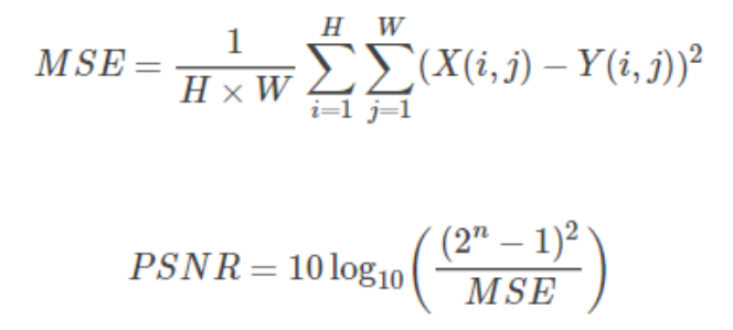
among ,n Is the number of bits per pixel .
PSNR Its unit is dB, The larger the value, the smaller the distortion , It is generally believed PSNR stay 38 The above time , The human eye cannot distinguish two pictures .
Related codes :
def psnr(loss):
    return 10 * log10(1 / loss.item())
5.2 SSIM
SSIM(Structural Similarity) For structural similarity , It consists of three comparison modules : brightness 、 Contrast 、 structure .
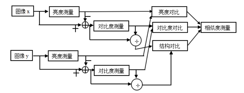
Brightness contrast function
Calculation formula of average gray level of image :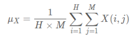
Calculation formula of brightness contrast function :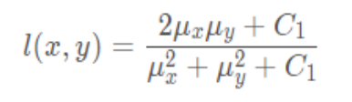
Contrast contrast function
Calculation formula of standard deviation of image :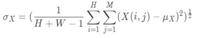
Calculation formula of contrast function :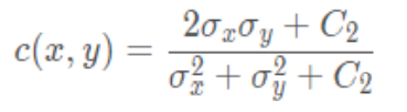
Structure comparison function
Structural comparison function calculation formula :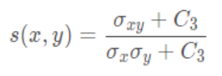
Combine the above three parts , obtain SSIM Calculation formula :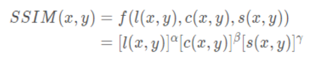
among , α \alpha α, β \beta β, γ \gamma γ > 0, To adjust the importance of these three modules .
SSIM The value range of the function is [0, 1], The larger the value, the smaller the image distortion , The more similar the two images are .
Related codes :
because pytorch There's nothing like tensorflow similar tf.image.ssim Calculate like this SSIM The interface of , Therefore, the user-defined function is used to calculate
"""  Calculation ssim function  """
#  Calculate one-dimensional Gaussian distribution vector
def gaussian(window_size, sigma):
    gauss = torch.Tensor(
        [exp(-(x - window_size//2)**2/float(2*sigma**2)) for x in range(window_size)])
    return gauss/gauss.sum()


#  Create Gaussian kernel , By matrix multiplication of two one-dimensional Gaussian distribution vectors
#  You can set channel The parameter is expanded to 3 passageway
def create_window(window_size, channel=1):
    _1D_window = gaussian(window_size, 1.5).unsqueeze(1)
    _2D_window = _1D_window.mm(
        _1D_window.t()).float().unsqueeze(0).unsqueeze(0)
    window = _2D_window.expand(
        channel, 1, window_size, window_size).contiguous()
    return window


#  Calculation SSIM
#  Use it directly SSIM Formula , But when calculating the mean , Instead of directly averaging pixels , Instead, normalized Gaussian kernel convolution is used to replace .
#  Formulas are used in calculating variance and covariance Var(X)=E[X^2]-E[X]^2, cov(X,Y)=E[XY]-E[X]E[Y].
def ssim(img1, img2, window_size=11, window=None, size_average=True, full=False, val_range=None):
    # Value range can be different from 255. Other common ranges are 1 (sigmoid) and 2 (tanh).
    if val_range is None:
        if torch.max(img1) > 128:
            max_val = 255
        else:
            max_val = 1

        if torch.min(img1) < -0.5:
            min_val = -1
        else:
            min_val = 0
        L = max_val - min_val
    else:
        L = val_range

    padd = 0
    (_, channel, height, width) = img1.size()
    if window is None:
        real_size = min(window_size, height, width)
        window = create_window(real_size, channel=channel).to(img1.device)

    mu1 = F.conv2d(img1, window, padding=padd, groups=channel)
    mu2 = F.conv2d(img2, window, padding=padd, groups=channel)

    mu1_sq = mu1.pow(2)
    mu2_sq = mu2.pow(2)
    mu1_mu2 = mu1 * mu2

    sigma1_sq = F.conv2d(img1 * img1, window, padding=padd,
                         groups=channel) - mu1_sq
    sigma2_sq = F.conv2d(img2 * img2, window, padding=padd,
                         groups=channel) - mu2_sq
    sigma12 = F.conv2d(img1 * img2, window, padding=padd,
                       groups=channel) - mu1_mu2

    C1 = (0.01 * L) ** 2
    C2 = (0.03 * L) ** 2

    v1 = 2.0 * sigma12 + C2
    v2 = sigma1_sq + sigma2_sq + C2
    cs = torch.mean(v1 / v2)  # contrast sensitivity

    ssim_map = ((2 * mu1_mu2 + C1) * v1) / ((mu1_sq + mu2_sq + C1) * v2)

    if size_average:
        ret = ssim_map.mean()
    else:
        ret = ssim_map.mean(1).mean(1).mean(1)

    if full:
        return ret, cs
    return ret


class SSIM(torch.nn.Module):
    def __init__(self, window_size=11, size_average=True, val_range=None):
        super(SSIM, self).__init__()
        self.window_size = window_size
        self.size_average = size_average
        self.val_range = val_range

        # Assume 1 channel for SSIM
        self.channel = 1
        self.window = create_window(window_size)

    def forward(self, img1, img2):
        (_, channel, _, _) = img1.size()

        if channel == self.channel and self.window.dtype == img1.dtype:
            window = self.window
        else:
            window = create_window(self.window_size, channel).to(
                img1.device).type(img1.dtype)
            self.window = window
            self.channel = channel

        return ssim(img1, img2, window=window, window_size=self.window_size, size_average=self.size_average)
6. model training / test
Set up epoch by 500 Time , Save on the validation set PSNR Highest model . The performance of the two models on the test set is shown in the following table :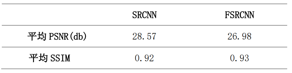
It can be found from the results that ,FSRCNN Of PSNR Than SRCNN low , but FSRCNN Of SSIM Than SRCNN high , explain PSNR and SSIM There is no completely positive correlation .
Training / Verification code :
model = FSRCNN(1).to(device)
criterion = nn.MSELoss()
optimizer = optim.Adam(model.parameters(), lr=1e-2)
scheduler = MultiStepLR(optimizer, milestones=[50, 75, 100], gamma=0.1)
best_psnr = 0.0
for epoch in range(nb_epochs):
    # Train
    epoch_loss = 0
    for iteration, batch in enumerate(trainloader):
        input, target = batch[0].to(device), batch[1].to(device)
        optimizer.zero_grad()
        out = model(input)
        loss = criterion(out, target)
        loss.backward()
        optimizer.step()
        epoch_loss += loss.item()
    print(f"Epoch {
      epoch}. Training loss: {
      epoch_loss / len(trainloader)}")
    # Val
    sum_psnr = 0.0
    sum_ssim = 0.0
    with torch.no_grad():
        for batch in valloader:
            input, target = batch[0].to(device), batch[1].to(device)
            out = model(input)
            loss = criterion(out, target)
            pr = psnr(loss)
            sm = ssim(input, out)
            sum_psnr += pr
            sum_ssim += sm
    print(f"Average PSNR: {
      sum_psnr / len(valloader)} dB.")
    print(f"Average SSIM: {
      sum_ssim / len(valloader)} ")
    avg_psnr = sum_psnr / len(valloader)
    if avg_psnr >= best_psnr:
        best_psnr = avg_psnr
        torch.save(model, r"best_model_FSRCNN.pth")
    scheduler.step()
Test code :
BATCH_SIZE = 4
model_path = "best_model_FSRCNN.pth"
testset = DatasetFromFolder(r"./data/images/test", zoom_factor)
testloader = DataLoader(dataset=testset, batch_size=BATCH_SIZE,
                        shuffle=False, num_workers=NUM_WORKERS)
sum_psnr = 0.0
sum_ssim = 0.0
model = torch.load(model_path).to(device)
criterion = nn.MSELoss()
with torch.no_grad():
    for batch in testloader:
        input, target = batch[0].to(device), batch[1].to(device)
        out = model(input)
        loss = criterion(out, target)
        pr = psnr(loss)
        sm = ssim(input, out)
        sum_psnr += pr
        sum_ssim += sm
print(f"Test Average PSNR: {
      sum_psnr / len(testloader)} dB")
print(f"Test Average SSIM: {
      sum_ssim / len(testloader)} ")
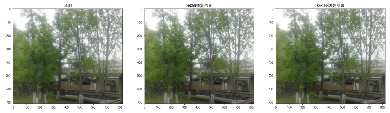
7. Real map test
In order to intuitively feel the effect of the two models , I use my own pictures to test the real pictures , The effect is as follows :
s=1( Magnification =1)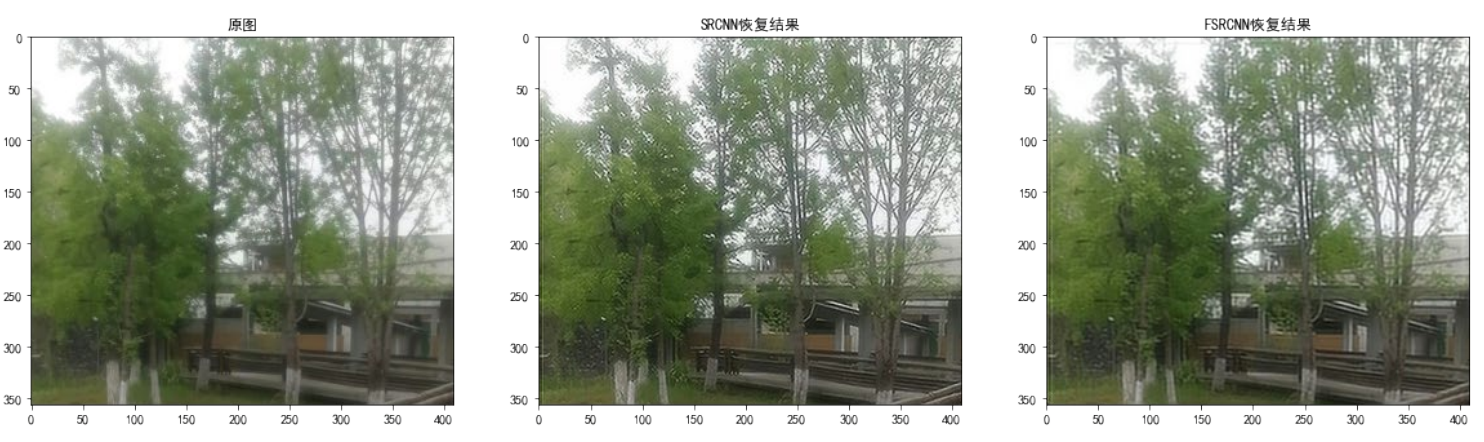
When the magnification =1 when ,SRCNN The super score result ratio of FSRCNN The super score effect of is better , This is on average with the two models PSNR The values of are consistent .
s=2( Magnification =2)
When the magnification =2 when ,SRCNN And FSRCNN There is little difference in the super score effect of .
Related codes :
#  Parameter setting
zoom_factor = 1
model = "best_model_SRCNN.pth"
model2 = "best_model_FSRCNN.pth"
image = "tree.png"
cuda = 'store_true'
device = torch.device("cuda:0" if torch.cuda.is_available() else "cpu")

#  Read the picture
img = Image.open(image).convert('YCbCr')
img = img.resize((int(img.size[0] * zoom_factor), int(img.size[1] * zoom_factor)), Image.BICUBIC)
y, cb, cr = img.split()
img_to_tensor = transforms.ToTensor()
input = img_to_tensor(y).view(1, -1, y.size[1], y.size[0]).to(device)

#  Output pictures
model = torch.load(model).to(device)
out = model(input).cpu()
out_img_y = out[0].detach().numpy()
out_img_y *= 255.0
out_img_y = out_img_y.clip(0, 255)
out_img_y = Image.fromarray(np.uint8(out_img_y[0]), mode='L')
out_img = Image.merge('YCbCr', [out_img_y, cb, cr]).convert('RGB')

model2 = torch.load(model2).to(device)
out2 = model2(input).cpu()
out_img_y2 = out2[0].detach().numpy()
out_img_y2 *= 255.0
out_img_y2 = out_img_y2.clip(0, 255)
out_img_y2 = Image.fromarray(np.uint8(out_img_y2[0]), mode='L')
out_img2 = Image.merge('YCbCr', [out_img_y2, cb, cr]).convert('RGB')

#  Drawing display
fig, ax = plt.subplots(1, 3, figsize=(20, 20))
ax[0].imshow(img)
ax[0].set_title(" Original picture ")
ax[1].imshow(out_img)
ax[1].set_title("SRCNN Recovery results ")
ax[2].imshow(out_img2)
ax[2].set_title("FSRCNN Recovery results ")
plt.show()
fig.savefig(r"tree2.png")
The source code for
Experimental report , Complete source code file , Data set acquisition :
https://download.csdn.net/download/qq1198768105/85906814
边栏推荐
- WebRTC 音频抗弱网技术(上)
- JSON解析实例(Qt含源码)
- With 8 modules and 40 thinking models, you can break the shackles of thinking and meet the thinking needs of different stages and scenes of your work. Collect it quickly and learn it slowly
- Ctfshow, information collection: web7
- [机缘参悟-40]:方向、规则、选择、努力、公平、认知、能力、行动,读3GPP 6G白皮书的五层感悟
- 【OBS】RTMPSockBuf_ Fill, remote host closed connection.
- 激光雷達lidar知識點滴
- Navigation - are you sure you want to take a look at such an easy-to-use navigation framework?
- Pinduoduo lost the lawsuit, and the case of bargain price difference of 0.9% was sentenced; Wechat internal test, the same mobile phone number can register two account functions; 2022 fields Awards an
- Niuke real problem programming - day15
猜你喜欢
Niuke real problem programming - Day11
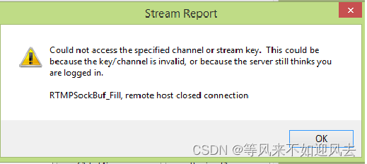
【OBS】RTMPSockBuf_Fill, remote host closed connection.
![[server data recovery] a case of RAID data recovery of a brand StorageWorks server](/img/aa/6d820d97e82df1d908dc7aa78fc8bf.png)
[server data recovery] a case of RAID data recovery of a brand StorageWorks server
暑期安全很重要!应急安全教育走进幼儿园
asp. Netnba information management system VS development SQLSERVER database web structure c programming computer web page source code project detailed design
CTFshow,信息搜集:web5

Deformable convolutional dense network for enhancing compressed video quality
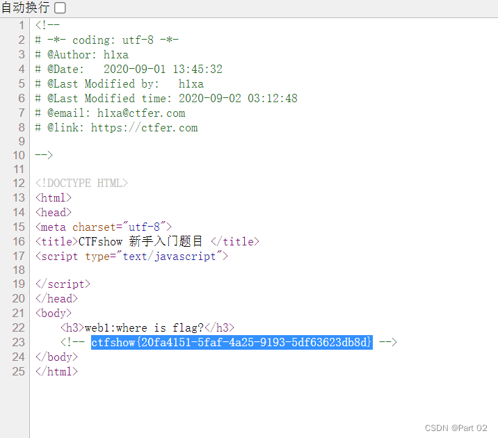
Ctfshow, information collection: web1
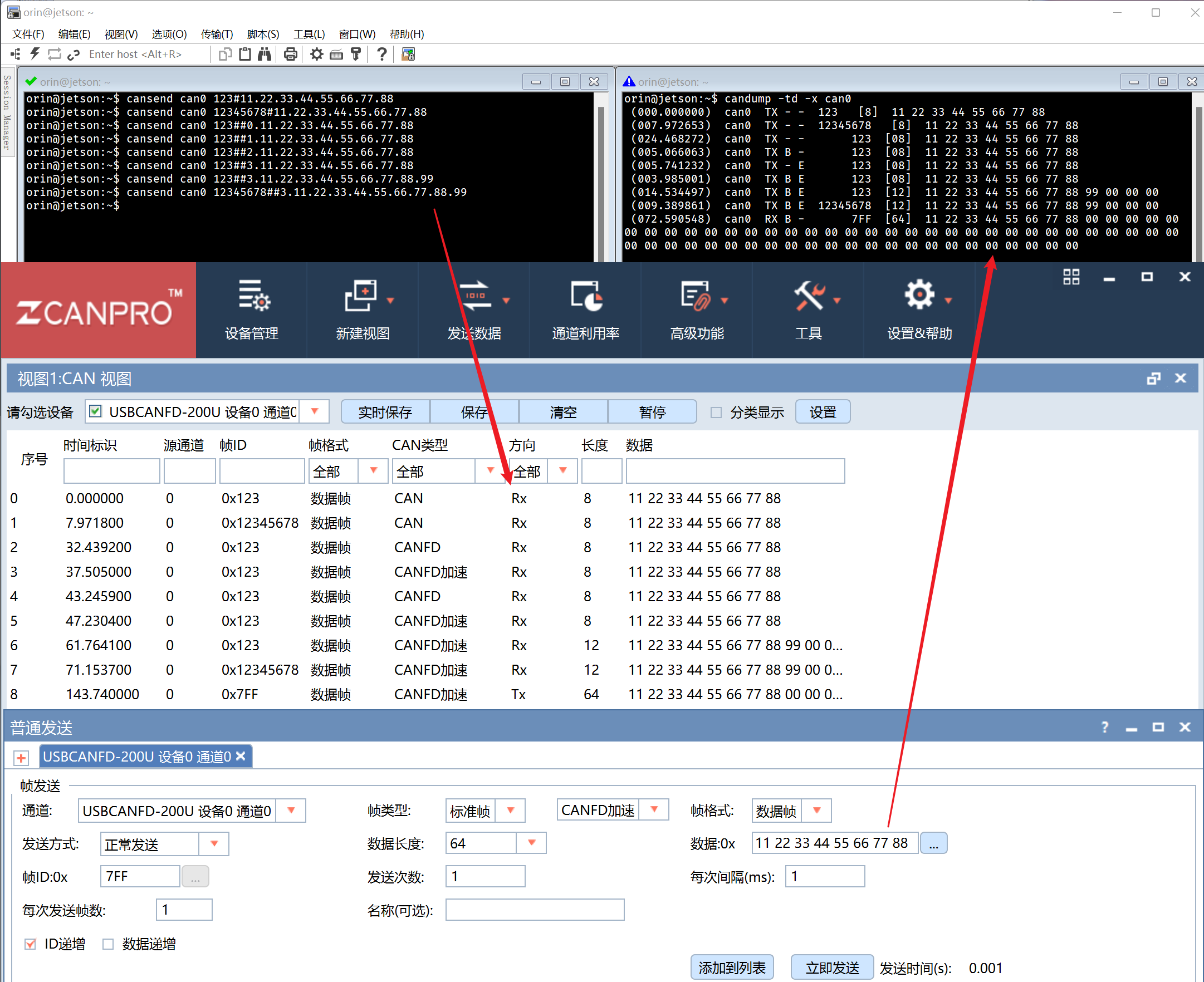
Used by Jetson AgX Orin canfd

Win10 or win11 taskbar, automatically hidden and transparent
随机推荐
智汀不用Home Assistant让小米智能家居接入HomeKit
数据库如何进行动态自定义排序?
一文读懂数仓中的pg_stat
Stream learning notes
Zhiting doesn't use home assistant to connect Xiaomi smart home to homekit
什么是pv和uv? pv、uv
Niuke real problem programming - Day9
Niuke real problem programming - Day12
#yyds干货盘点# 解决名企真题:交叉线
asp. Netnba information management system VS development SQLSERVER database web structure c programming computer web page source code project detailed design
Ctfshow, information collection: web4
什麼是數據泄露
Shengteng experience officer Episode 5 notes I
Niuke real problem programming - Day17
【OBS】RTMPSockBuf_ Fill, remote host closed connection.
MySQL installation configuration 2021 in Windows Environment
知否|两大风控最重要指标与客群好坏的关系分析
Guangzhou Development Zone enables geographical indication products to help rural revitalization
6. Electron borderless window and transparent window lock mode setting window icon
众昂矿业:萤石继续引领新能源市场增长