Watermelon book learning notes - Chapter 4 decision tree

One 、 The basic process of decision-making learning

1.1 Basic definition of decision tree

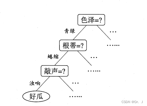
The decision tree is mainly composed of root nodes 、 Internal nodes and leaf nodes , In addition to the classification results corresponding to leaf nodes , Both the root node and the internal node correspond to an attribute test , Each node can contain several sample sets , These samples will be divided into child nodes according to the test results of the node , And the ultimate goal of decision tree is to learn a strong generalization ability

1.1.1 The root node

Include all training samples , And the path from the root node to each leaf node represents a complete prediction process

1.1.2 Internal node

The internal node will contain a subset of all samples , And the internal node can use a single attribute as the basis for attribute testing , You can also train classifiers in internal nodes to improve generalization ability

1.1.3 Leaf node

What leaf nodes contain is the final prediction result , For example, two classification tasks , The value of leaves is 0/1, And leaf nodes can contain sample sets or It's OK not to include

1.1.4 Diagram of decision tree

1.1.5 The training process of decision tree algorithm

When the following three situations occur , The decision tree cannot be divided

1. The sample categories contained in the current node are the same , At this time, there is no need to divide
2. Property set is empty , That is, the attribute set completes the division task , Or all samples have the same value on all attributes , Without division
3. No training samples in node , Can't divide

NOTE: When you encounter the second situation , Directly turn this node into a leaf node , On the determination of category , It is divided according to the largest proportion of sample categories in this node , For example, there are more good melons than bad ones in the sample , Set it as a good melon node ;
In the third case, it is also set as a leaf node , However, when determining the category, it should be determined according to its parent node , The specific method is the same as that in the second case

Two 、 Partition attribute selection

The optimal partition attribute is the key to the success of decision tree algorithm

2.1 Relevant concepts

1. Information entropy
It is mainly used to measure the purity in the sample set . The greater the entropy of information , Explain the data set D The lower the purity of . Hypothetical data set D pass the civil examinations k The proportion of class samples is pk, Then we can get the following formula of information entropy , among |y| Refers to the number of types of samples ,Ent（D） For datasets D The entropy of information

Note: The maximum value of information entropy is log2|y|, The minimum value is 0
2. Information gain
Information gain is mainly used to measure whether an attribute can be used as a partition attribute for the next partition of the decision tree , Is a very important measure . Generally speaking , The larger the information gain value obtained , It indicates that this attribute is more suitable as a partition attribute . The calculation method is as follows , among a Indicates the partition attribute ,Dv Represents in the sample set D In attribute a The upper value is av A collection of samples ,v And attribute a The number of values is equal ：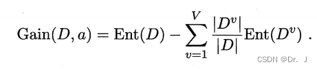

See the watermelon book for specific calculation cases p76
3. Gain rate
The reason why the gain rate appears is that the information gain is biased towards the attributes with more attribute values in the formula calculation results , Therefore, the concept of gain rate appears to measure the division effect of attributes , The symbolic representation of the formula and the calculation of information gain are the same ：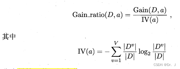

Note:

1. IV(a) Attribute a The intrinsic value of , attribute a The more you can get , The larger the intrinsic value
2. In fact, the calculation result of the gain rate is biased towards the attributes with a small number of values , So the famous decision tree algorithm C4.5 It is not directly used as a division measurement index , The method it uses is to calculate the information gain of each attribute first , Then calculate the average , Pick out attributes that are greater than the average information gain level , Then filter the final partition attributes through the gain rate

4. gini index
This concept was first used in CART Decision leaf Algorithm [Breiman et al., 1984], In this algorithm, the purity of data set is not expressed by information entropy , Instead, use the Gini value , As follows ：

It can be seen from the formula , The Gini value is calculated in a sample , The probability of two different samples appearing at the same time , So the smaller the Gini index , The probability of different samples appearing at the same time is smaller , That means the higher the purity of the data set , So it further leads to properties a Gini index calculation formula ：

Note: When selecting the optimal partition attribute , Choose the lowest Gini index as the partition attribute

2.2 Case studies

Refer to the case of watermelon book , It's very detailed

3、 ... and 、 Pruning

Because machine learning algorithm has the possibility of fitting , Therefore, over fitting of decision tree is unavoidable , If the data set of the decision tree is divided too carefully in the training process , It will lead to more branches of the decision tree , The decision tree will learn some special attributes from the training samples , Eventually, it will lead to over fitting and reduce the generalization ability , Pruning is an effective method to alleviate over fitting in decision tree algorithm

3.1 pre-pruning

3.1.1 The main process ：

When dividing the decision tree , Evaluate the progressiveness of each node before dividing , Judge whether this node division can improve the generalization ability of the decision tree

3.1.2 The calculation process

See watermelon book for detailed process p81

3.1.3 Advantages and disadvantages of pre pruning

1. advantage
   It can effectively reduce the risk of over fitting , And fewer branches can make the training and testing time of decision tree shorter
2. shortcoming
   It may make some branches that can improve the generalization ability of the decision tree unable to expand in the subsequent division , This will bring the risk of under fitting to the decision tree

3.2 After pruning

3.2.1 The main process ：

First, use the training set to generate a decision tree , Then start with the non leaf nodes at the bottom , Calculate whether replacing the non leaf node with leaf node can bring generalization improvement to the decision tree

3.2.2 The calculation process

Watermelon book p82 And the corresponding chapters of pumpkin book

3.2.3 Advantages and disadvantages of post pruning

1. advantage
   Because it is a bottom-up pruning operation , So we will keep as many branches as possible , Basically, it will not lead to under fitting , Therefore, the generalization ability of decision tree after post pruning is usually stronger than that of pre pruning
2. shortcoming
   Test the performance impact of non leaf nodes from bottom to top , The cost of post pruning is much higher

Four 、 Continuous and missing values

4.1 The processing of continuous values in decision tree

The main idea
Discretize continuous attributes

4.1.1 Dichotomy discretization of continuous values

Methods described
With data set D And continuous properties a, For example, the density and sweetness of watermelon are continuous attributes ,a In the data D There are several values on , Write it down as {α1,α2, . . , an }. Based on dividing points t You can put D It is divided into two subsets containing positive and negative samples , namely t Threshold value . For partition points t, We can take such a set

each t Are the average values of two adjacent attribute values , In this way, we can t Equal to the attribute value in discrete case . Based on this, the information gain calculation formula is changed to the following formula , Choose the one that maximizes the information gain t As a dividing point .

4.1.2 Specific calculation

See watermelon book for the calculation process p85 Corresponding chapters to pumpkin book

4.2 Processing of missing values

Two main problems

1. How to select partition attributes when attribute values are missing
2. Given partition properties , If the value of the sample on the attribute is missing , How to divide the samples

4.2.1 Related definitions

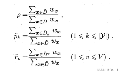
among , Pair attribute α, ρ The proportion of samples without missing values in the table , Pk Indicates that there is no missing value in the sample , The first k The proportion of classes rv It means that there is no missing value in the attribute α Top value av The proportion of the sample of .

4.2.2 The generalized information gain formula for dealing with missing values

The definition of symbols in the formula is the same as the previous formula

4.2.3 Solution of two problems

1. The solution of the first problem
   First, find out the sample subset of the original data set that has no missing values on the selected attributes D1, problem 1 It can be done by D1 To calculate the information gain
2. The second question is
   If the value of the sample in the division attribute is not missing , Then keep the weight unchanged ,（ The weight is in the previous definition w, And the initial is 1）, And put it into the child node of the corresponding category
   If the value of the sample on the partition attribute is missing , Then divide this sample into all child nodes , Then update its weight , Turn it into rv*w, Its essence is to divide the sample into sub nodes with different probabilities

4.2.4 The calculation process

See watermelon book p88 Corresponding chapters to pumpkin book

5、 ... and 、 Multivariate decision trees

5.1 Classification boundary of decision tree

The attribute of the sample can be regarded as a coordinate axis in space , The sample is mapped to N A numerical point in dimensional space , Therefore, the classification task for the whole data set is equivalent to finding a suitable classification boundary . The classification boundary of decision tree has its own judgment characteristics , Each classification boundary is parallel to the coordinate axis , Here's the picture

The classification boundary obtained in the above figure is based on the following decision tree

Therefore, we can see that the classification boundary of the decision tree can correspond well with the attributes , But when the judgment process is complex , Using this expression will cause huge expenses

5.2 Multivariable decision tree with oblique boundary

describe
In a multivariable decision tree , The interior of a non leaf node can be more than just an attribute , It can also be a trainer , Like a neural network , Or a perceptron , Or a linear classifier , These models can be trained by the data set contained in these non leaf nodes , So in multivariable decision tree , The learning task becomes the training of classifiers
Example
The following figure is a decision tree composed of a simple linear classifier

This is its classification boundary

Can see , Multivariable decision tree can effectively improve the situation that the classification boundary of univariate decision tree is parallel to the coordinate axis