当前位置:网站首页>Formula understanding in quadruped control
Formula understanding in quadruped control
2022-06-26 08:33:00 【Yu Getou】
- explain : This article is used to record the formula understanding of quadruped related papers , Due to my limited ability , The understanding of the formula comes from studying the content of the paper , A combination of online articles and personal guesses , You are welcome to criticize and correct any inaccuracies , This article will also be updated . Welcome to contact me :[email protected]
《MIT Cheetah 3: Design and Control of a Robust, Dynamic Quadruped Robot》
1. Support leg controller
(1) Based on the centralized quality model (lumped model) Balance controller for (Balance Controller)
i. The motion equation of the robot which regards the robot as a single rigid body model :
[ I 3 … I 3 [ p 1 p c ] × … [ p 4 p c ] × ] ⏟ A F = [ m ( p ¨ c + g ) I G ω b ˙ ] ⏟ b \underbrace{\begin{bmatrix} I_3 &\dots & I_3 \\ [p_1 p_c]\times &\dots &[p_4 p_c]\times \end{bmatrix}}_{A} F=\underbrace{\begin{bmatrix} m(\ddot{p}_c+g )\\ I_G\dot{\omega _b} \end{bmatrix}}_b A[I3[p1pc]×……I3[p4pc]×]F=b[m(p¨c+g)IGωb˙]
Using the basic Newton's laws of motion
- Together = ma
- Resultant moment = inertia * Angular acceleration
ii. Use PD The control law calculates the centroid acceleration and angular acceleration
[ p ¨ c , d ω ˙ b , d ] = [ K p , p ( p c , d − p c ) + K d , p ( p ˙ c , d − p ˙ c ) K p , ω log ( R d R T ) + K d , ω ( ω b , d − ω ) ] \left[\begin{array}{c} \ddot{\boldsymbol{p}}_{c, d} \\ \dot{\boldsymbol{\omega}}_{b, d} \end{array}\right]=\left[\begin{array}{c} \boldsymbol{K}_{p, p}\left(\boldsymbol{p}_{c, d}-\boldsymbol{p}_{c}\right)+\boldsymbol{K}_{d, p}\left(\dot{\boldsymbol{p}}_{c, d}-\dot{\boldsymbol{p}}_{c}\right) \\ \boldsymbol{K}_{p, \omega} \log \left(\boldsymbol{R}_{d} \boldsymbol{R}^{T}\right)+\boldsymbol{K}_{d, \omega}\left(\boldsymbol{\omega}_{b, d}-\boldsymbol{\omega}\right) \end{array}\right] [p¨c,dω˙b,d]=[Kp,p(pc,d−pc)+Kd,p(p˙c,d−p˙c)Kp,ωlog(RdRT)+Kd,ω(ωb,d−ω)]
The goal is : Get the optimal control force F, Make the center of mass tend to the ideal center of mass dynamic state
b d = [ m ( p ¨ c , d + g ) I G ω ˙ b , d ] \boldsymbol{b_d} = \begin{bmatrix} m(\ddot{\boldsymbol{p}}_{c,d}+\boldsymbol{g})\\ \boldsymbol{I_G}\dot{\boldsymbol{\omega}}_{b,d} \end{bmatrix} bd=[m(p¨c,d+g)IGω˙b,d]
Because the robot motion equation is linear , The optimization problem can be transformed into QP problem
F ∗ = min F ∈ R 12 ( A F − b d ) T S ( A F − b d ) + α ∣ ∣ F ∣ ∣ 2 + β ∣ ∣ F − F p r e v ∣ ∣ 2 s . t . C F ≤ d \boldsymbol{F^*}=\min_{F\in R^{12}} \quad (AF-b_d)^TS(AF-b_d)+\alpha ||F||^2+\beta || F-F_{prev}||^2\\ s.t. \quad CF\le d F∗=F∈R12min(AF−bd)TS(AF−bd)+α∣∣F∣∣2+β∣∣F−Fprev∣∣2s.t.CF≤d
significance :
- ( A F − b d ) T S ( A F − b d ) (AF-b_d)^TS(AF-b_d) (AF−bd)TS(AF−bd) ---- Make the center of mass state meet the expectation ,S The matrix represents the priority of rotation and displacement in the control .
- ∣ ∣ F ∣ ∣ 2 ||F||^2 ∣∣F∣∣2 ---- Minimize the force
- ∣ ∣ F − F p r e v ∣ ∣ 2 ||F-F_{prev}||^2 ∣∣F−Fprev∣∣2 ---- F p r e v F_{prev} Fprev Represents the last force in the iteration , The goal is to limit the difference between the solutions of the two iterations .
- α , β > 0 \alpha,\beta>0 α,β>0 ---- Specify the standardization of knowledge , And filter the solution to some extent .
- C F ≤ d CF\le d CF≤d ---- The details are unknown , The purpose is to ensure that the solution is in the feasible region .
(2)MPC controller (Model Predictive Control)
J = ∑ i = 0 k ( x i − x i r e f ) T Q i ( x i − x i r e f ) + u i T R i u i J=\sum_{i=0}^{k}(x_i-x_i^{ref})^TQ_i(x_i-x_i^{ref})+u_i^TR_iu_i J=i=0∑k(xi−xiref)TQi(xi−xiref)+uiTRiui
The goal is : Constantly updated u i u_i ui Input to the control system , Minimize the above cost function .
- The update frequency f: In this paper, the optimal solution is given by 30Hz The frequency of is input to the controller
- Solving process : Paper points out , Need to put MPC Problem into QP Solve the problem .
MPC For details of the controller, please refer to my study notes :MPC Learning notes
2. Swing leg controller
(1) Foot drop point calculation
p s t e p , i = p h , i + T c ϕ 2 p ˙ c , d ⏟ R a i b e r t H e u r i s t i c + z 0 ∣ ∣ g ∣ ∣ ( p ˙ c − p ˙ c , d ) ⏟ C a p t u r e P o i n t p_{step,i}=p_{h,i}+\underbrace{\frac{T_{c_\phi}}{2}{\dot{p}}_{c,d}}_{Raibert \ Heuristic}+\underbrace{\sqrt{\frac{z_0}{||g||}}({\dot{p}}_c-{\dot{p}}_{c,d})}_{Capture \ Point} pstep,i=ph,i+Raibert Heuristic2Tcϕp˙c,d+Capture Point∣∣g∣∣z0(p˙c−p˙c,d)
T c ϕ 2 p ˙ c , d \frac{T_{c_\phi}}{2}{\dot{p}}_{c,d} 2Tcϕp˙c,d ---- according to 《Legged robots that balance》 Description in , The landing point of the foot end determined according to the formula , Will make the motion symmetrical , Acceleration is 0
z 0 ∣ ∣ g ∣ ∣ ( p ˙ c − p ˙ c , d ) \sqrt{\frac{z_0}{||g||}}({\dot{p}}_c-{\dot{p}}_{c,d}) ∣∣g∣∣z0(p˙c−p˙c,d) ---- according to 《Capture point: A step toward humanoid push recovery》 Description in , The goal is to make the foothold closer capture point, At this point the legs will be balanced .
T c φ T_{c_\varphi} Tcφ ---- In an ideal state stance State duration
z 0 z_0 z0 ---- The height of the target location point
p h , i p_{h,i} ph,i---- leg i Corresponding hip motor hip The location of
(2) Swing trajectory calculation –PD controller + Feedforward control
i. Calculation of feedforward torque
τ f f , i = J i ⊤ Λ i ( B a i , ref − J ˙ i q ˙ i ) + C i q ˙ i + G i \tau_{\mathrm{ff}, i}=\boldsymbol{J}_{i}^{\top} \boldsymbol{\Lambda}_{i}\left({ }^{\mathfrak{B}} \boldsymbol{a}_{i, \text { ref }}-\dot{\boldsymbol{J}}_{i} \dot{\boldsymbol{q}}_{i}\right)+\boldsymbol{C}_{i} \dot{\boldsymbol{q}}_{i}+\boldsymbol{G}_{i} τff,i=Ji⊤Λi(Bai, ref −J˙iq˙i)+Ciq˙i+Gi
J i J_i Ji ---- Jacobian matrix of the foot
Λ i \Lambda _i Λi ---- Inertia matrix of operation space
B a i , r e f ^\mathfrak{B}a_{i,ref} Bai,ref ---- Reference acceleration
q i q_i qi ---- Vector of joint structure
C i C_i Ci ---- Coriolis matrix
G i G_i Gi ----- Heavy moment
ii. Track following controller
τ i = J i ⊤ [ K p ( B p i , ref − B p i ) + K d ( B v i , r e f − B v i ) ] + τ f f , i \boldsymbol{\tau}_{i}=\boldsymbol{J}_{i}^{\top}\left[\boldsymbol{K}_{p}\left({ }^{\mathfrak{B}} \boldsymbol{p}_{i, \text { ref }}-{ }^{\mathfrak{B}} \boldsymbol{p}_{i}\right)+\boldsymbol{K}_{d}\left({ }^{\mathfrak{B}} \boldsymbol{v}_{i, \mathrm{ref}}-{^\mathfrak{B}} \boldsymbol{v}_{i}\right)\right]+\boldsymbol{\tau}_{\mathrm{ff}, i} τi=Ji⊤[Kp(Bpi, ref −Bpi)+Kd(Bvi,ref−Bvi)]+τff,i
- Control frequency f:4.5kHz
In order to make PD The controller remains stable , You need to adjust the gain K p K_{p} Kp Do the following
K p , j = ω d e s 2 Λ j j ( q ) K_{p,j}=\omega_{des}^2\Lambda_{jj}(q) Kp,j=ωdes2Λjj(q)
- K p , j K_{p,j} Kp,j ---- K p K_p Kp No j Diagonal terms .
- ω d e s \omega_{des} ωdes ---- Target natural frequency
- Λ j j \Lambda_{jj} Λjj ---- The first j Inertia matrix of diagonal terms in operation space
3. Virtual Prediction supports polygons (Virtual Predictive Support Polygon)
i. Calculate the weight factor for each leg
(1) Virtual support polygon : Provide centroid position points under various gait
(2) Define the contribution of each leg to the prediction polygon ( Phase by phase ): Point out which leg should be raised or touched , And the time of state switching
K c ϕ = 1 2 [ erf ( ϕ σ c 0 2 ) + erf ( 1 − ϕ σ c 1 2 ) ] K c ˉ ϕ = 1 2 [ 2 + erf ( − ϕ σ c ˉ 0 2 ) + erf ( ϕ − 1 σ c ˉ 1 2 ) ] Φ = s ϕ K c ϕ + s ˉ ϕ K c ˉ ϕ \begin{array}{r} K_{c_{\phi}}=\frac{1}{2}\left[\operatorname{erf}\left(\frac{\phi}{\sigma_{c_{0}} \sqrt{2}}\right)+\operatorname{erf}\left(\frac{1-\phi}{\sigma_{c_{1}} \sqrt{2}}\right)\right] \\\\ K_{\bar{c}_{\phi}}=\frac{1}{2}\left[2+\operatorname{erf}\left(\frac{-\phi}{\sigma_{\bar{c}_{0}} \sqrt{2}}\right)+\operatorname{erf}\left(\frac{\phi-1}{\sigma_{\bar{c}_{1}} \sqrt{2}}\right)\right] \\\\ \Phi=s_{\phi} K_{c_{\phi}}+\bar{s}_{\phi} K_{\bar{c}_{\phi}} \end{array} Kcϕ=21[erf(σc02ϕ)+erf(σc121−ϕ)]Kcˉϕ=21[2+erf(σcˉ02−ϕ)+erf(σcˉ12ϕ−1)]Φ=sϕKcϕ+sˉϕKcˉϕ
e r f ( x ) erf(x) erf(x) ---- Gaussian error function
K c ϕ , K c ˉ ϕ K_{c_{\phi}},K_{\bar{c}_{\phi}} Kcϕ,Kcˉϕ ---- Weight factor of support phase and swing phase
Φ \Phi Φ ---- The total weight factor of the leg
meaning : In the supported state , The closer a leg is to the center , The more it can be used as a support point , Under the dynamic pendulum , The closer a leg is to the center , The less it can be used to balance
ii. Calculate the virtual points of each leg
[ ξ i − ξ i + ] = [ p i p i − p i p i + ] [ Φ i 1 − Φ i ] \left[\begin{array}{c} \boldsymbol{\xi}_{i}^{-} \\ \boldsymbol{\xi}_{i}^{+} \end{array}\right]=\left[\begin{array}{ll} \boldsymbol{p}_{i} & \boldsymbol{p}_{i^{-}} \\ \boldsymbol{p}_{i} & \boldsymbol{p}_{i^{+}} \end{array}\right]\left[\begin{array}{c} \Phi_{i} \\ 1-\Phi_{i} \end{array}\right] [ξi−ξi+]=[pipipi−pi+][Φi1−Φi]
- A positive superscript indicates counterclockwise , A negative superscript indicates clockwise
iii. Calculate the predicted polygon vertices for each leg
ξ i = Φ i p i + Φ i ξ i − + Φ i + ξ i + Φ i + Φ i − + Φ i + \boldsymbol{\xi}_{i}=\frac{\Phi_{i} \boldsymbol{p}_{i}+\Phi_{i} \boldsymbol{\xi}_{i}^{-}+\Phi_{i+} \boldsymbol{\xi}_{i}^{+}}{\Phi_{i}+\Phi_{i^{-}}+\Phi_{i^{+}}} ξi=Φi+Φi−+Φi+Φipi+Φiξi−+Φi+ξi+
iv. Calculate the desired centroid position
p ^ C o M , d = 1 N ∑ i = 1 N ξ i \hat{\boldsymbol{p}}_{C o M, d}=\frac{1}{N} \sum_{i=1}^{N} \boldsymbol{\xi}_{i} p^CoM,d=N1i=1∑Nξi
4. Attitude adjustment in sloping terrain
meaning : Represents a plane , That is, the plane where the quadruped robot is currently located
z ( x , y ) = a 0 + a 1 x + a 2 y z(x, y)=a_{0}+a_{1} x+a_{2} y z(x,y)=a0+a1x+a2y
meaning : Get a plane according to the current state of the robot , namely a={ a 0 , a 1 , a 2 a_0,a_1,a_2 a0,a1,a2}
a = ( W T W ) † W T p z W = [ 1 p x p y ] 4 × 3 \begin{aligned} \boldsymbol{a} &=\left(\boldsymbol{W}^{T} \boldsymbol{W}\right)^{\dagger} \boldsymbol{W}^{T} \boldsymbol{p}^{z} \\ \boldsymbol{W} &=\left[\begin{array}{lll} \mathbf{1} & \boldsymbol{p}^{x} & \boldsymbol{p}^{y} \end{array}\right]_{4 \times 3} \end{aligned} aW=(WTW)†WTpz=[1pxpy]4×3
- p x , p y , p z \boldsymbol{p^x},\boldsymbol{p^y},\boldsymbol{p^z} px,py,pz ---- Including the status of each leg of the robot , such as p x = ( p 1 x , p 2 x , p 3 x , p 4 x ) \boldsymbol{p^x} = (p_1^x,p_2^x,p_3^x,p_4^x) px=(p1x,p2x,p3x,p4x)
5. State estimation
It uses Kalman filtering and Extended Kalman filter , I won't elaborate here .
《Highly Dynamic Quadruped Locomotion via Whole-Body Impulse Control and Model Predictive Control》
1. Hybrid controller
The goal is : Split the position control into two simple controllers to control
(1)MPC controller
m p ¨ = ∑ i = 1 n c f i − c g , d d t ( I ω ) = ∑ i = 1 n c r i × f i \begin{array}{l} m \ddot{\mathbf{p}}=\sum_{i=1}^{n_{c}} \mathbf{f}_{i}-\mathbf{c}_{g}, \\\\ \frac{d}{d t}(\boldsymbol{I} \boldsymbol{\omega})=\sum_{i=1}^{n_{c}} \mathbf{r}_{i} \times \mathbf{f}_{i} \end{array} mp¨=∑i=1ncfi−cg,dtd(Iω)=∑i=1ncri×fi
- Similar to the above balance controller , Objects are Lumped mass model , But here we use MPC To find the optimal control force .
(2)WBIC controller (Whole-Body Impulse Control)
A ( q ¨ f q ¨ j ) + b + g = ( 0 6 τ ) + J c ⊤ f r \boldsymbol{A}\left(\begin{array}{c} \ddot{\mathbf{q}}_{f} \\ \ddot{\mathbf{q}}_{j} \end{array}\right)+\mathbf{b}+\mathbf{g}=\left(\begin{array}{c} \mathbf{0}_{6} \\ \boldsymbol{\tau} \end{array}\right)+\boldsymbol{J}_{c}^{\top} \mathbf{f}_{r} A(q¨fq¨j)+b+g=(06τ)+Jc⊤fr
A A A ---- quality ( inertia ) matrix
b b b ---- Coriolis force
g g g ---- gravity
τ \tau τ ---- Joint torque
f r f_r fr ---- Increased force
J c J_c Jc ---- Jacobian matrix of touchdown point
Understanding of iterative formulas
Reference resources Hand push WBC The formula
Continuous updating …
边栏推荐
- Vs2019-mfc setting edit control and static text font size
- Using transformers of hugging face to realize text classification
- ZLMediaKit推流拉流测试
- STM32 porting mpu6050/9250 DMP official library (motion_driver_6.12) modifying and porting DMP simple tutorial
- CodeBlocks集成Objective-C开发
- Zlib static library compilation
- 2020-10-29
- Ltp-- extract time, person and place
- Esp8266wifi module tutorial: punctual atom atk-esp8266 for network communication, single chip microcomputer and computer, single chip microcomputer and mobile phone to send data
- Calculation of decoupling capacitance
猜你喜欢

【Unity Mirror】NetworkTeam的使用

HEVC学习之码流分析
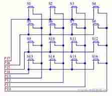
(5) Matrix key
![[postgraduate entrance examination] group planning exercises: memory](/img/ac/5c63568399f68910a888ac91e0400c.png)
[postgraduate entrance examination] group planning exercises: memory

Opencv learning notes II

Can the encrypted JS code and variable name be cracked and restored?

Use a switch to control the lighting and extinguishing of LEP lamp

OpenCV Learning notes iii
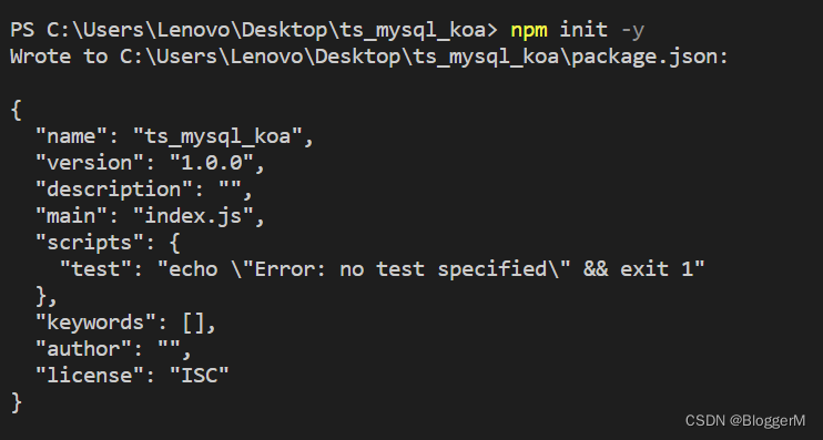
Koa_mySQL_Ts 的整合

"System error 5 occurred when win10 started mysql. Access denied"
随机推荐
利用无线技术实现分散传感器信号远程集中控制
Relation extraction model -- spit model
Opencv learning notes 3
First character that appears only once
Two ways to realize time format printing
Learning signal integrity from scratch (SIPI) -- 3 challenges faced by Si and Si based design methods
Implementation of ffmpeg audio and video player
VS2005 compiles libcurl to normaliz Solution of Lib missing
static const与static constexpr的类内数据成员初始化
Text to SQL model ----irnet
软件工程-个人作业-提问回顾与个人总结
STM32 project design: temperature, humidity and air quality alarm, sharing source code and PCB
Introduction of laser drive circuit
2020-10-17
Interpretation of x-vlm multimodal model
Relationship extraction -- casrel
Addition of attention function in yolov5
Win10 mysql-8.0.23-winx64 solution for forgetting MySQL password (detailed steps)
Esp8266wifi module tutorial: punctual atom atk-esp8266 for network communication, single chip microcomputer and computer, single chip microcomputer and mobile phone to send data
Design of reverse five times voltage amplifier circuit