"Analysis of 43 cases of MATLAB neural network": Chapter 42 parallel operation and neural network - parallel neural network operation based on cpu/gpu

1. Preface

《MATLAB neural network 43 A case study 》 yes MATLAB Technology Forum （www.matlabsky.com） planning , Led by teacher wangxiaochuan ,2013 Beijing University of Aeronautics and Astronautics Press MATLAB A book for tools MATLAB Example teaching books , Is in 《MATLAB neural network 30 A case study 》 On the basis of modification 、 Complementary , Adhering to “ Theoretical explanation — case analysis — Application extension ” This feature , Help readers to be more intuitive 、 Learn neural networks vividly .

《MATLAB neural network 43 A case study 》 share 43 Chapter , The content covers common neural networks （BP、RBF、SOM、Hopfield、Elman、LVQ、Kohonen、GRNN、NARX etc. ） And related intelligent algorithms （SVM、 Decision tree 、 Random forests 、 Extreme learning machine, etc ）. meanwhile , Some chapters also cover common optimization algorithms （ Genetic algorithm (ga) 、 Ant colony algorithm, etc ） And neural network . Besides ,《MATLAB neural network 43 A case study 》 It also introduces MATLAB R2012b New functions and features of neural network toolbox in , Such as neural network parallel computing 、 Custom neural networks 、 Efficient programming of neural network, etc .

In recent years, with the rise of artificial intelligence research , The related direction of neural network has also ushered in another upsurge of research , Because of its outstanding performance in the field of signal processing , The neural network method is also being applied to various applications in the direction of speech and image , This paper combines the cases in the book , It is simulated and realized , It's a relearning , I hope I can review the old and know the new , Strengthen and improve my understanding and practice of the application of neural network in various fields . I just started this book on catching more fish , Let's start the simulation example , Mainly to introduce the source code application examples in each chapter , This paper is mainly based on MATLAB2018a(64 position ,MATLAB2015b Parallel processing toolkit is not installed ) Platform simulation implementation , This is the example of parallel operation and neural network in Chapter 42 of this book , Don't talk much , Start ！

2. MATLAB Simulation example 1

open MATLAB, Click on “ Home page ”, Click on “ open ”, Find the sample file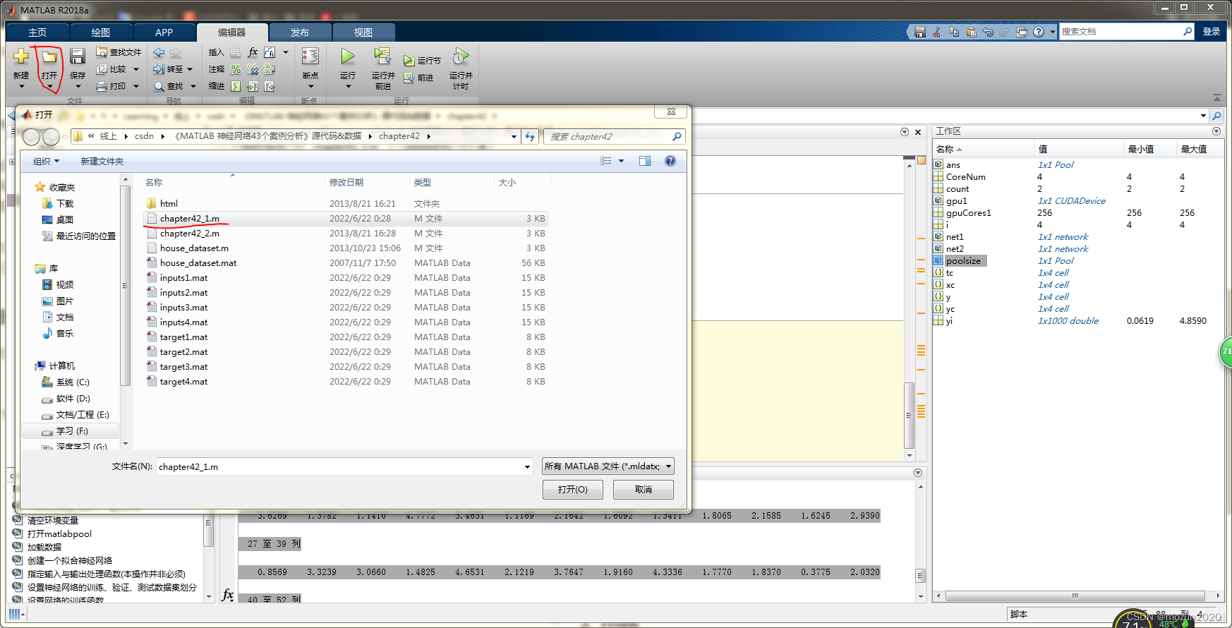

Choose chapter42_1.m, Click on “ open ”

chapter42_1.m Source code is as follows ：

%%%%%%%%%%%%%%%%%%%%%%%%%%%%%%%%%%%%%%%%%%%%%%%%%%%%
% function ： Parallel operation and neural network - be based on CPU/GPU Parallel neural network operation based on 
% Environmental Science ：Win7,Matlab2015b
%Modi: C.S
% Time ：2022-06-21
%%%%%%%%%%%%%%%%%%%%%%%%%%%%%%%%%%%%%%%%%%%%%%%%%%%%


%% Matlab neural network 43 A case study 

%  Parallel operation and neural network - be based on CPU/GPU Parallel neural network operation based on 
% by  Wang Xiao Chuan (@ Wang Xiao Chuan _matlab)
% http://www.matlabsky.com
% Email:[email protected]163.com
% http://weibo.com/hgsz2003
%  This code is a sample code script , It is recommended not to operate as a whole , Pay attention to notes during operation .
close all;
clear all 
clc

tic
%% CPU parallel 
%%  Standard single thread neural network training and simulation process 
[x,t]=house_dataset;
net1=feedforwardnet(10);
net2=train(net1,x,t);
y=sim(net2,x);

%%  open MATLAB workers
% matlabpool open

%  Check worker Number 
delete(gcp('nocreate'))
poolsize=parpool(2)

%%  Set up train And sim Parameters in function “Useparallel” by “yes”.
net2=train(net1,x,t,'Useparallel','yes')
y=sim(net2,x,'Useparallel','yes');

%%  Use “showResources” Options confirm that neural network operations are indeed in various worker Up operation .
net2=train(net1,x,t,'useParallel','yes','showResources','yes');
y=sim(net2,x,'useParallel','yes','showResources','yes');

%%  Divide a data set randomly , Save to different files at the same time 
CoreNum=2; % Set up the machine CPU The core number 
if isempty(gcp('nocreate'))
    parpool(CoreNum);
end
for i=1:2
x=rand(2,1000);
save(['inputs' num2str(i)],'x')
t=x(1,:).*x(2,:)+2*(x(1,:)+x(2,:)) ;
save(['target' num2str(i)],'t');
clear x t
end

%%  Realize parallel operation and load data set 　
CoreNum=2; % Set up the machine CPU The core number 
if isempty(gcp('nocreate'))
    parpool(CoreNum);
end
for i=1:2
    data=load(['inputs' num2str(i)],'x');
    xc{
    i}=data.x;
    data=load(['target' num2str(i)],'t');
    tc{
    i}=data.t;
    clear data
end
net2=configure(net2,xc{
    1},tc{
    1});
net2=train(net2,xc,tc);
yc=sim(net2,xc);

%%  Get each one worker Back to Composite result 
CoreNum=2; % Set up the machine CPU The core number 
if isempty(gcp('nocreate'))
    parpool(CoreNum);
end
for i=1:2
    yi=yc{
    i};
end

%% GPU parallel 
count=gpuDeviceCount
gpu1=gpuDevice(1)
gpuCores1=gpu1.MultiprocessorCount*gpu1.SIMDWidth
net2=train(net1,xc,tc,'useGPU','yes')
y=sim(net2,xc,'useGPU','yes')
net1.trainFcn='trainscg';
net2=train(net1,xc,tc,'useGPU','yes','showResources','yes');
y=sim(net2,xc, 'useGPU','yes','showResources','yes');
toc

Add completed , Click on “ function ”, Start emulating , The output simulation results are as follows ：

Parallel pool using the 'local' profile is shutting down.
Starting parallel pool (parpool) using the 'local' profile ...
connected to 2 workers.

poolsize = 

 Pool -  attribute : 

            Connected: true
           NumWorkers: 2
              Cluster: local
        AttachedFiles: {
    }
    AutoAddClientPath: true
          IdleTimeout: 30 minutes (30 minutes remaining)
          SpmdEnabled: true


net2 =

    Neural Network
 
              name: 'Feed-Forward Neural Network'
          userdata: (your custom info)
 
    dimensions:
 
         numInputs: 1
         numLayers: 2
        numOutputs: 1
    numInputDelays: 0
    numLayerDelays: 0
 numFeedbackDelays: 0
 numWeightElements: 151
        sampleTime: 1
 
    connections:
 
       biasConnect: [1; 1]
      inputConnect: [1; 0]
      layerConnect: [0 0; 1 0]
     outputConnect: [0 1]
 
    subobjects:
 
             input: Equivalent to inputs{
    1}
            output: Equivalent to outputs{
    2}
 
            inputs: {
    1x1 cell array of 1 input}
            layers: {
    2x1 cell array of 2 layers}
           outputs: {
    1x2 cell array of 1 output}
            biases: {
    2x1 cell array of 2 biases}
      inputWeights: {
    2x1 cell array of 1 weight}
      layerWeights: {
    2x2 cell array of 1 weight}
 
    functions:
 
          adaptFcn: 'adaptwb'
        adaptParam: (none)
          derivFcn: 'defaultderiv'
         divideFcn: 'dividerand'
       divideParam: .trainRatio, .valRatio, .testRatio
        divideMode: 'sample'
           initFcn: 'initlay'
        performFcn: 'mse'
      performParam: .regularization, .normalization
          plotFcns: {
    'plotperform', plottrainstate, ploterrhist,
                    plotregression}
        plotParams: {
    1x4 cell array of 4 params}
          trainFcn: 'trainlm'
        trainParam: .showWindow, .showCommandLine, .show, .epochs,
                    .time, .goal, .min_grad, .max_fail, .mu, .mu_dec,
                    .mu_inc, .mu_max
 
    weight and bias values:
 
                IW: {
    2x1 cell} containing 1 input weight matrix
                LW: {
    2x2 cell} containing 1 layer weight matrix
                 b: {
    2x1 cell} containing 2 bias vectors
 
    methods:
 
             adapt: Learn while in continuous use
         configure: Configure inputs & outputs
            gensim: Generate Simulink model
              init: Initialize weights & biases
           perform: Calculate performance
               sim: Evaluate network outputs given inputs
             train: Train network with examples
              view: View diagram
       unconfigure: Unconfigure inputs & outputs
 
 
Computing Resources:
Parallel Workers:
  Worker 1 on 123-PC, MEX on PCWIN64
  Worker 2 on 123-PC, MEX on PCWIN64
 
 
Computing Resources:
Parallel Workers:
  Worker 1 on 123-PC, MEX on PCWIN64
  Worker 2 on 123-PC, MEX on PCWIN64
 

count =

     2


gpu1 = 

  CUDADevice -  attribute :

                      Name: 'GeForce GTX 960'
                     Index: 1
         ComputeCapability: '5.2'
            SupportsDouble: 1
             DriverVersion: 10.2000
            ToolkitVersion: 9
        MaxThreadsPerBlock: 1024
          MaxShmemPerBlock: 49152
        MaxThreadBlockSize: [1024 1024 64]
               MaxGridSize: [2.1475e+09 65535 65535]
                 SIMDWidth: 32
               TotalMemory: 4.2950e+09
           AvailableMemory: 3.2666e+09
       MultiprocessorCount: 8
              ClockRateKHz: 1266000
               ComputeMode: 'Default'
      GPUOverlapsTransfers: 1
    KernelExecutionTimeout: 1
          CanMapHostMemory: 1
           DeviceSupported: 1
            DeviceSelected: 1


gpuCores1 =

   256

NOTICE: Jacobian training not supported on GPU. Training function set to TRAINSCG.

net2 =

    Neural Network
 
              name: 'Feed-Forward Neural Network'
          userdata: (your custom info)
 
    dimensions:
 
         numInputs: 1
         numLayers: 2
        numOutputs: 1
    numInputDelays: 0
    numLayerDelays: 0
 numFeedbackDelays: 0
 numWeightElements: 41
        sampleTime: 1
 
    connections:
 
       biasConnect: [1; 1]
      inputConnect: [1; 0]
      layerConnect: [0 0; 1 0]
     outputConnect: [0 1]
 
    subobjects:
 
             input: Equivalent to inputs{
    1}
            output: Equivalent to outputs{
    2}
 
            inputs: {
    1x1 cell array of 1 input}
            layers: {
    2x1 cell array of 2 layers}
           outputs: {
    1x2 cell array of 1 output}
            biases: {
    2x1 cell array of 2 biases}
      inputWeights: {
    2x1 cell array of 1 weight}
      layerWeights: {
    2x2 cell array of 1 weight}
 
    functions:
 
          adaptFcn: 'adaptwb'
        adaptParam: (none)
          derivFcn: 'defaultderiv'
         divideFcn: 'dividerand'
       divideParam: .trainRatio, .valRatio, .testRatio
        divideMode: 'sample'
           initFcn: 'initlay'
        performFcn: 'mse'
      performParam: .regularization, .normalization
          plotFcns: {
    'plotperform', plottrainstate, ploterrhist,
                    plotregression}
        plotParams: {
    1x4 cell array of 4 params}
          trainFcn: 'trainscg'
        trainParam: .showWindow, .showCommandLine, .show, .epochs,
                    .time, .goal, .min_grad, .max_fail, .sigma,
                    .lambda
 
    weight and bias values:
 
                IW: {
    2x1 cell} containing 1 input weight matrix
                LW: {
    2x2 cell} containing 1 layer weight matrix
                 b: {
    2x1 cell} containing 2 bias vectors
 
    methods:
 
             adapt: Learn while in continuous use
         configure: Configure inputs & outputs
            gensim: Generate Simulink model
              init: Initialize weights & biases
           perform: Calculate performance
               sim: Evaluate network outputs given inputs
             train: Train network with examples
              view: View diagram
       unconfigure: Unconfigure inputs & outputs
 

y =

  1×2 cell  Array 

    {
    1×1000 double}    {
    1×1000 double}

 
Computing Resources:
GPU device #1, GeForce GTX 960
 
 
Computing Resources:
GPU device #1, GeForce GTX 960
 
 Time has passed  70.246120  second .

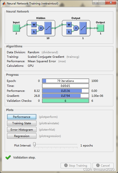
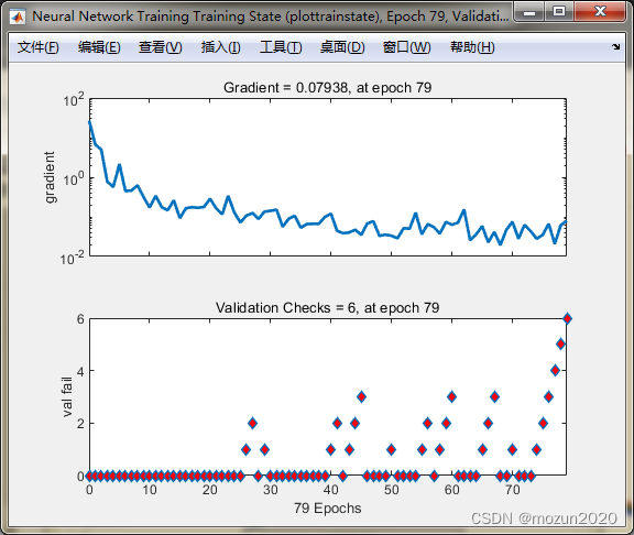
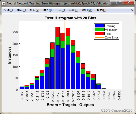
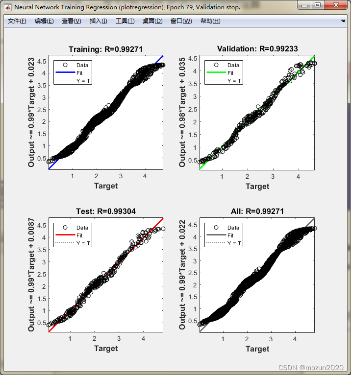
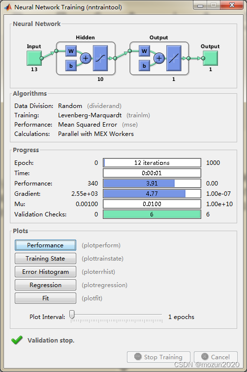
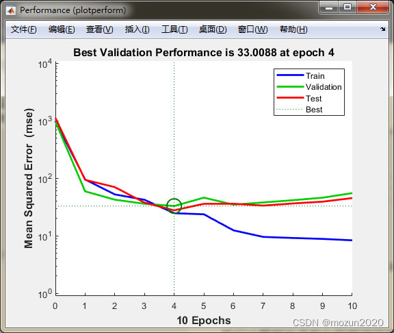
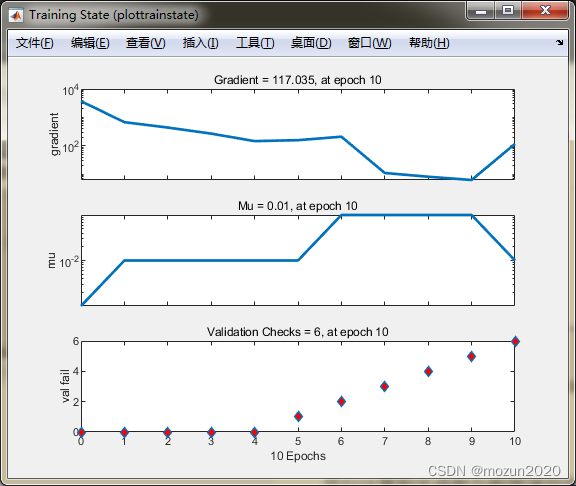
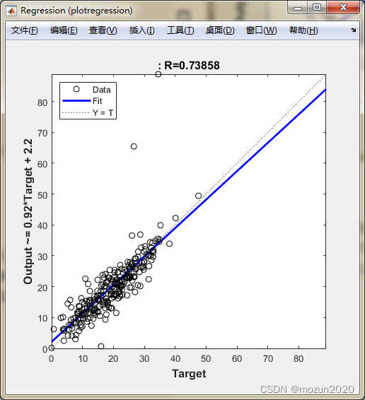
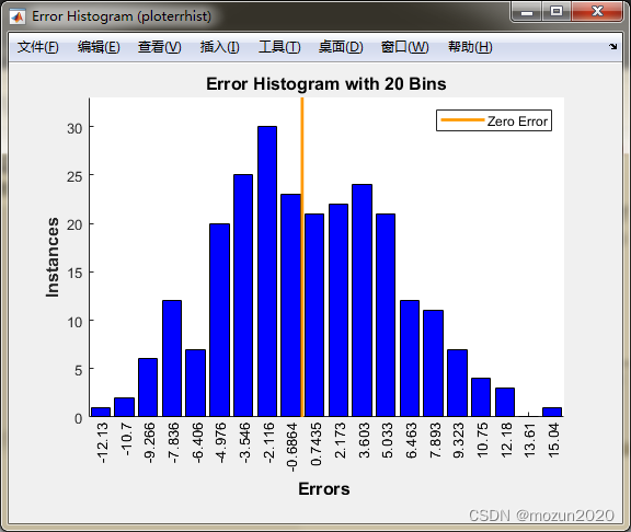
In turn, click Plots Medium Performance,Training State,Error Histogram,Regression The following figure can be obtained ：

3. MATLAB Simulation example 2

Select and open MATLAB In the current folder view chapter42_2.m,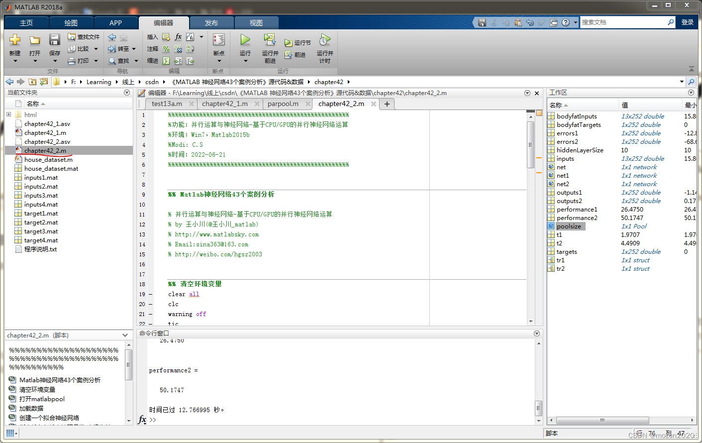

chapter42_2.m Source code is as follows ：

%%%%%%%%%%%%%%%%%%%%%%%%%%%%%%%%%%%%%%%%%%%%%%%%%%%%
% function ： Parallel operation and neural network - be based on CPU/GPU Parallel neural network operation based on 
% Environmental Science ：Win7,Matlab2015b
%Modi: C.S
% Time ：2022-06-21
%%%%%%%%%%%%%%%%%%%%%%%%%%%%%%%%%%%%%%%%%%%%%%%%%%%%


%% Matlab neural network 43 A case study 

%  Parallel operation and neural network - be based on CPU/GPU Parallel neural network operation based on 
% by  Wang Xiao Chuan (@ Wang Xiao Chuan _matlab)
% http://www.matlabsky.com
% Email:[email protected]163.com
% http://weibo.com/hgsz2003
 

%%  Clear environment variables 
clear all
clc
warning off
tic
%%  open matlabpool
% matlabpool open
delete(gcp('nocreate'))
poolsize=parpool(2)

%%  Load data 
load bodyfat_dataset
inputs = bodyfatInputs;
targets = bodyfatTargets;

%%  Create a fitting neural network 
hiddenLayerSize = 10;   %  The number of neurons in the hidden layer is 10
net = fitnet(hiddenLayerSize);  %  Creating networks 

%%  Specify input and output processing functions ( This operation is not necessary )
net.inputs{
    1}.processFcns = {
    'removeconstantrows','mapminmax'};
net.outputs{
    2}.processFcns = {
    'removeconstantrows','mapminmax'};

%%  Set up the training of neural network 、 verification 、 Test data set partitioning 
net.divideFcn = 'dividerand';  %  Randomly divide the data set 
net.divideMode = 'sample';  %   The division unit is each data 
net.divideParam.trainRatio = 70/100; % Training set ratio 
net.divideParam.valRatio = 15/100; % Verification set ratio 
net.divideParam.testRatio = 15/100; % Test set ratio 

%%  Set the training function of the network 
net.trainFcn = 'trainlm';  % Levenberg-Marquardt

%%  Set the error function of the network 
net.performFcn = 'mse';  % Mean squared error

%%  Set the network visualization function 
net.plotFcns = {
    'plotperform','plottrainstate','ploterrhist', ...
  'plotregression', 'plotfit'};

%%  Single thread network training 
tic
[net1,tr1] = train(net,inputs,targets);
t1=toc;
disp([' The training time of single thread neural network is ',num2str(t1),' second ']);

%%  Parallel network training 
tic
[net2,tr2] = train(net,inputs,targets,'useParallel','yes','showResources','yes');
t2=toc;
disp([' The training time of the parallel neural network is ',num2str(t2),' second ']);

%%  Network effect verification 
outputs1 = sim(net1,inputs);
outputs2 = sim(net2,inputs);
errors1 = gsubtract(targets,outputs1);
errors2 = gsubtract(targets,outputs2);
performance1 = perform(net1,targets,outputs1);
performance2 = perform(net2,targets,outputs2);

%%  Neural network visualization 
figure, plotperform(tr1);
figure, plotperform(tr2);
figure, plottrainstate(tr1);
figure, plottrainstate(tr2);
figure,plotregression(targets,outputs1);
figure,plotregression(targets,outputs2);
figure,ploterrhist(errors1);
figure,ploterrhist(errors2);
toc
% matlabpool close

Click on “ function ”, Start emulating , The output simulation results are as follows ：

Parallel pool using the 'local' profile is shutting down.
Starting parallel pool (parpool) using the 'local' profile ...
connected to 2 workers.

poolsize = 

 Pool -  attribute : 

            Connected: true
           NumWorkers: 2
              Cluster: local
        AttachedFiles: {
    }
    AutoAddClientPath: true
          IdleTimeout: 30 minutes (30 minutes remaining)
          SpmdEnabled: true

 The training time of single thread neural network is 1.9707 second 
 
Computing Resources:
Parallel Workers:
  Worker 1 on 123-PC, MEX on PCWIN64
  Worker 2 on 123-PC, MEX on PCWIN64
 
 The training time of the parallel neural network is 4.4909 second 

performance1 =

   26.4750


performance2 =

   50.1747

 Time has passed  12.766995  second .

4. Summary

Parallel computing related functions and data calls are in MATLAB2015 There are upgrades after version , So we need to adjust the source code and then simulate , The examples in this article are based on the situation of the machine and MATLAB Version adaptation . Interested in the content of this chapter or want to fully learn and understand , It is suggested to study the contents of chapter 42 in the book . Some of these knowledge points will be supplemented on the basis of their own understanding in the later stage , Welcome to study and exchange together .