当前位置:网站首页>《MATLAB 神经网络43个案例分析》:第41章 定制神经网络的实现——神经网络的个性化建模与仿真
《MATLAB 神经网络43个案例分析》:第41章 定制神经网络的实现——神经网络的个性化建模与仿真
2022-07-02 03:21:00 【mozun2020】
《MATLAB 神经网络43个案例分析》:第41章 定制神经网络的实现——神经网络的个性化建模与仿真
1. 前言
《MATLAB 神经网络43个案例分析》是MATLAB技术论坛(www.matlabsky.com)策划,由王小川老师主导,2013年北京航空航天大学出版社出版的关于MATLAB为工具的一本MATLAB实例教学书籍,是在《MATLAB神经网络30个案例分析》的基础上修改、补充而成的,秉承着“理论讲解—案例分析—应用扩展”这一特色,帮助读者更加直观、生动地学习神经网络。
《MATLAB神经网络43个案例分析》共有43章,内容涵盖常见的神经网络(BP、RBF、SOM、Hopfield、Elman、LVQ、Kohonen、GRNN、NARX等)以及相关智能算法(SVM、决策树、随机森林、极限学习机等)。同时,部分章节也涉及了常见的优化算法(遗传算法、蚁群算法等)与神经网络的结合问题。此外,《MATLAB神经网络43个案例分析》还介绍了MATLAB R2012b中神经网络工具箱的新增功能与特性,如神经网络并行计算、定制神经网络、神经网络高效编程等。
近年来随着人工智能研究的兴起,神经网络这个相关方向也迎来了又一阵研究热潮,由于其在信号处理领域中的不俗表现,神经网络方法也在不断深入应用到语音和图像方向的各种应用当中,本文结合书中案例,对其进行仿真实现,也算是进行一次重新学习,希望可以温故知新,加强并提升自己对神经网络这一方法在各领域中应用的理解与实践。自己正好在多抓鱼上入手了这本书,下面开始进行仿真示例,主要以介绍各章节中源码应用示例为主,本文主要基于MATLAB2015b(32位)平台仿真实现,这是本书第四十一章定制神经网络的实现实例,话不多说,开始!
2. MATLAB 仿真示例
打开MATLAB,点击“主页”,点击“打开”,找到示例文件
选中chapter41.m,点击“打开”
chapter41.m源码如下:
%%%%%%%%%%%%%%%%%%%%%%%%%%%%%%%%%%%%%%%%%%%%%%%%%%%%
%功能:定制神经网络的实现-神经网络的个性化建模与仿真
%环境:Win7,Matlab2015b
%Modi: C.S
%时间:2022-06-21
%%%%%%%%%%%%%%%%%%%%%%%%%%%%%%%%%%%%%%%%%%%%%%%%%%%%
%% Matlab神经网络43个案例分析
% 定制神经网络的实现-神经网络的个性化建模与仿真
% by 王小川(@王小川_matlab)
% http://www.matlabsky.com
% Email:[email protected]163.com
% http://weibo.com/hgsz2003
%% 清空环境变量
clear all
clc
warning off
tic
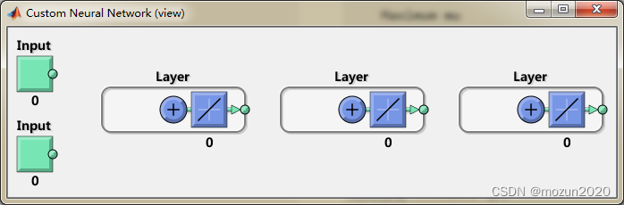
%% 建立一个“空”神经网络
net = network
%% 输入与网络层数定义
net.numInputs = 2;
net.numLayers = 3;
%% 使用view(net)观察神经网络结构。
view(net)
% 此时神经网络有两个输入,三个神经元层。但请注意:net.numInputs设置的是
% 神经网络的输入个数,每个输入的维数是由net.inputs{
i}.size控制。
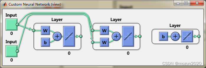
%% 阈值连接定义
net.biasConnect(1) = 1;
net.biasConnect(3) = 1;
% 或者使用net.biasConnect = [1; 0; 1];
view(net)
%% 输入与层连接定义
net.inputConnect(1,1) = 1;
net.inputConnect(2,1) = 1;
net.inputConnect(2,2) = 1;
% 或者使用net.inputConnect = [1 0; 1 1; 0 0];
view(net)
net.layerConnect = [0 0 0; 0 0 0; 1 1 1];
view(net)
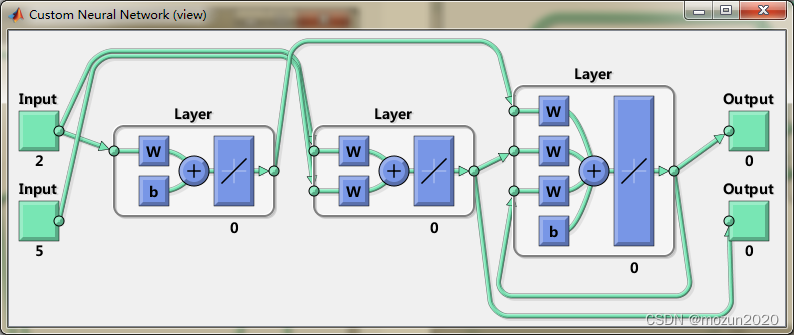
%% 输出连接设置
net.outputConnect = [0 1 1];
view(net)
%% 输入设置
net.inputs
net.inputs{
1}
net.inputs{
1}.processFcns = {
'removeconstantrows','mapminmax'};
net.inputs{
2}.size = 5;
net.inputs{
1}.exampleInput = [0 10 5; 0 3 10];
view(net)
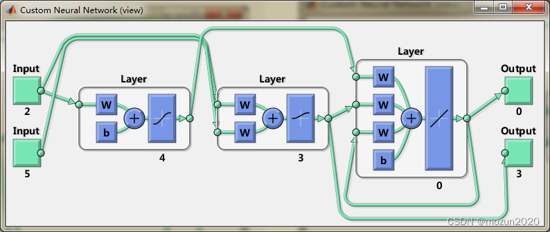
%% 层设置
net.layers{
1}
% 将神经网络第一层的神经元个数设置为4个,其传递函数设置为“tansig”并
% 将其初始化函数设置为Nguyen-Widrow函数。
net.layers{
1}.size = 4;
net.layers{
1}.transferFcn = 'tansig';
net.layers{
1}.initFcn = 'initnw';
% 将第二层神经元个数设置为3个,其传递函数设置为“logsig”,并使用“initnw”初始化。
net.layers{
2}.size = 3;
net.layers{
2}.transferFcn = 'logsig';
net.layers{
2}.initFcn = 'initnw';
% 将第三层初始化函数设置为“initnw”
net.layers{
3}.initFcn = 'initnw';
view(net)
%% 输出设置
net.outputs
net.outputs{
2}
%% 阈值,输入权值与层权值设置
net.biases
net.biases{
1}
net.inputWeights
net.layerWeights
%% 将神经网络的某些权值的延迟进行设置
net.inputWeights{
2,1}.delays = [0 1];
net.inputWeights{
2,2}.delays = 1;
net.layerWeights{
3,3}.delays = 1;
%% 网络函数设置
% 将神经网络初始化设置为“initlay”,这样神经网络就可以按照
% 我们设置的层初始化函数“ initnw”即Nguyen-Widrow进行初始化。
net.initFcn = 'initlay';
% 将神经网络的误差设置为“mse”(mean squared error),同时将神经网络的训练函数
% 设置为“trainlm”Levenberg-Marquardt backpropagation)。
net.performFcn = 'mse';
net.trainFcn = 'trainlm';
% 为了使神经网络可以随机划分训练数据集,我们可以将divideFcn设置为“dividerand”。
net.divideFcn = 'dividerand';
% 将 plot functions设置为:“plotperform”,“plottrainstate”
net.plotFcns = {
'plotperform','plottrainstate'};
%% 权值阈值大小设置
net.IW{
1,1}, net.IW{
2,1}, net.IW{
2,2}
net.LW{
3,1}, net.LW{
3,2}, net.LW{
3,3}
net.b{
1}, net.b{
3}
%% 神经网络初始化
net = init(net);
net.IW{
1,1}
%% 神经网络的训练
X = {
[0; 0] [2; 0.5]; [2; -2; 1; 0; 1] [-1; -1; 1; 0; 1]};
T = {
[1; 1; 1] [0; 0; 0]; 1 -1};
Y = sim(net,X)
%% 神经网络的训练参数
net.trainParam
%% 训练网络
net = train(net,X,T);
%% 仿真来检查神经网络是否相应正常。
Y = sim(net,X)
toc
添加完毕,点击“运行”,开始仿真,输出仿真结果如下:
net =

    Neural Network

              name: 'Custom Neural Network'
          userdata: (your custom info)

    dimensions:

         numInputs: 0
         numLayers: 0
        numOutputs: 0
    numInputDelays: 0
    numLayerDelays: 0
 numFeedbackDelays: 0
 numWeightElements: 0
        sampleTime: 1

    connections:

       biasConnect: []
      inputConnect: []
      layerConnect: []
     outputConnect: []

    subobjects:

            inputs: {
    0x1 cell array of 0 inputs}
            layers: {
    0x1 cell array of 0 layers}
           outputs: {
    1x0 cell array of 0 outputs}
            biases: {
    0x1 cell array of 0 biases}
      inputWeights: {
    0x0 cell array of 0 weights}
      layerWeights: {
    0x0 cell array of 0 weights}

    functions:

          adaptFcn: (none)
        adaptParam: (none)
          derivFcn: 'defaultderiv'
         divideFcn: (none)
       divideParam: (none)
        divideMode: 'sample'
           initFcn: 'initlay'
        performFcn: 'mse'
      performParam: .regularization, .normalization
          plotFcns: {
    }
        plotParams: {
    1x0 cell array of 0 params}
          trainFcn: (none)
        trainParam: (none)

    weight and bias values:

                IW: {
    0x0 cell} containing 0 input weight matrices
                LW: {
    0x0 cell} containing 0 layer weight matrices
                 b: {
    0x1 cell} containing 0 bias vectors

    methods:

             adapt: Learn while in continuous use
         configure: Configure inputs & outputs
            gensim: Generate Simulink model
              init: Initialize weights & biases
           perform: Calculate performance
               sim: Evaluate network outputs given inputs
             train: Train network with examples
              view: View diagram
       unconfigure: Unconfigure inputs & outputs


ans =

    [1x1 nnetInput]
    [1x1 nnetInput]


ans =

    Neural Network Input

              name: 'Input'
    feedbackOutput: []
       processFcns: {
    }
     processParams: {
    1x0 cell array of 0 params}
   processSettings: {
    0x0 cell array of 0 settings}
    processedRange: []
     processedSize: 0
             range: []
              size: 0
          userdata: (your custom info)


ans =

    Neural Network Layer

              name: 'Layer'
        dimensions: 0
       distanceFcn: (none)
     distanceParam: (none)
         distances: []
           initFcn: 'initwb'
       netInputFcn: 'netsum'
     netInputParam: (none)
         positions: []
             range: []
              size: 0
       topologyFcn: (none)
       transferFcn: 'purelin'
     transferParam: (none)
          userdata: (your custom info)


ans =

    []    [1x1 nnetOutput]    [1x1 nnetOutput]


ans =

    Neural Network Output

              name: 'Output'
     feedbackInput: []
     feedbackDelay: 0
      feedbackMode: 'none'
       processFcns: {
    }
     processParams: {
    1x0 cell array of 0 params}
   processSettings: {
    0x0 cell array of 0 settings}
    processedRange: [3x2 double]
     processedSize: 3
             range: [3x2 double]
              size: 3
          userdata: (your custom info)


ans =

    [1x1 nnetBias]
    []
    [1x1 nnetBias]


ans =

    Neural Network Bias

           initFcn: (none)
             learn: true
          learnFcn: (none)
        learnParam: (none)
              size: 4
          userdata: (your custom info)


ans =

    [1x1 nnetWeight]                  []
    [1x1 nnetWeight]    [1x1 nnetWeight]
                  []                  []


ans =

                  []                  []                  []
                  []                  []                  []
    [1x1 nnetWeight]    [1x1 nnetWeight]    [1x1 nnetWeight]


ans =

     0     0
     0     0
     0     0
     0     0


ans =

     0     0     0     0
     0     0     0     0
     0     0     0     0


ans =

     0     0     0     0     0
     0     0     0     0     0
     0     0     0     0     0


ans =

   空矩阵: 0×4


ans =

   空矩阵: 0×3


ans =

     []


ans =

     0
     0
     0
     0


ans =

   空矩阵: 0×1


ans =

    1.9468    2.0124
    2.3881   -1.4619
   -1.7285    2.2028
   -0.2749    2.7865


Y =

    [3x1 double]    [3x1 double]
    [0x1 double]    [0x1 double]


ans =


    Function Parameters for 'trainlm'

    Show Training Window Feedback   showWindow: true
    Show Command Line Feedback showCommandLine: false
    Command Line Frequency                show: 25
    Maximum Epochs                      epochs: 1000
    Maximum Training Time                 time: Inf
    Performance Goal                      goal: 0
    Minimum Gradient                  min_grad: 1e-07
    Maximum Validation Checks         max_fail: 6
    Mu                                      mu: 0.001
    Mu Decrease Ratio                   mu_dec: 0.1
    Mu Increase Ratio                   mu_inc: 10
    Maximum mu                          mu_max: 10000000000


Y =

    [3x1 double]    [3x1 double]
    [    1.0000]    [   -1.0000]

时间已过 3.932652 秒。


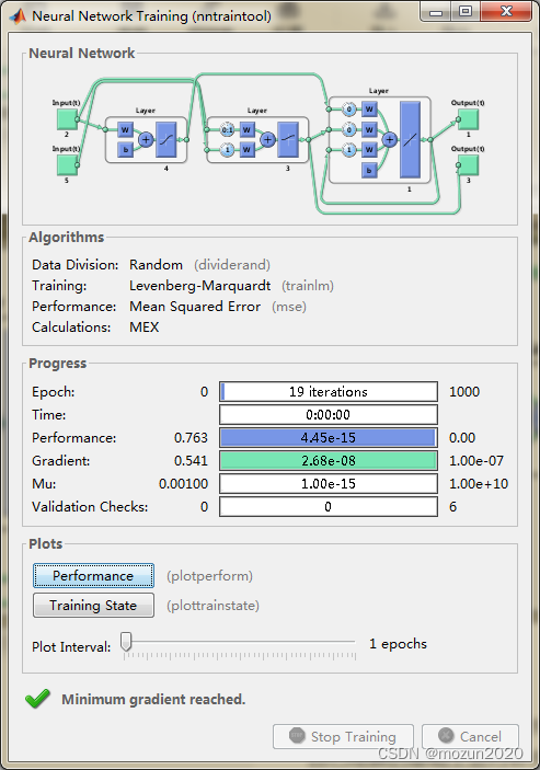
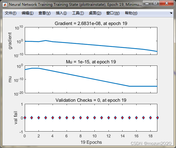
依次点击Plots中的Performance,Training State可得以下图示: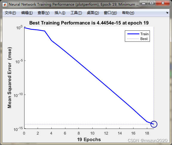
3. 小结
本章介绍了定制神经网络的方法,包括如何设置网络,如何链接网络,并通过对输入输出,连接阈值,输入的连接,输出的连接等进行相应设置,从而得到自己所需的神经网络,再导入数据进行相应的训练,得到模型后再进行预测检验,一个完整的定制神经网络的过程即已实现。对本章内容感兴趣或者想充分学习了解的,建议去研习书中第四十一章节的内容。后期会对其中一些知识点在自己理解的基础上进行补充,欢迎大家一起学习交流。
边栏推荐
- ZABBIX API creates hosts in batches according to the host information in Excel files
- Principle of computer composition - interview questions for postgraduate entrance examination (review outline, key points and reference)
- MySQL advanced (Advanced) SQL statement (II)
- ORA-01547、ORA-01194、ORA-01110
- MMSegmentation系列之训练与推理自己的数据集(三)
- Find duplicates [Abstract binary / fast and slow pointer / binary enumeration]
- JS introduction < 1 >
- West digital decided to raise the price of flash memory products immediately after the factory was polluted by materials
- 2022 hoisting machinery command examination paper and summary of hoisting machinery command examination
- Yan Rong looks at how to formulate a multi cloud strategy in the era of hybrid cloud
猜你喜欢

Named block Verilog

How to develop digital collections? How to develop your own digital collections
Redis cluster
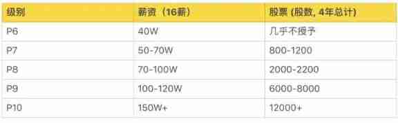
A list of job levels and salaries in common Internet companies. Those who have conditions must enter big factories. The salary is really high

Baohong industry | 6 financial management models at different stages of life

Xiaomi, a young engineer, was just going to make soy sauce

图扑软件通过 CMMI5 级认证!| 国际软件领域高权威高等级认证
Verilog 时序控制
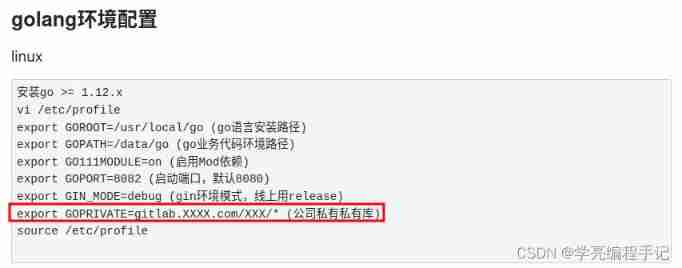
Golang configure export goprivate to pull private library code

QT environment generates dump to solve abnormal crash
随机推荐
Docker installs canal and MySQL for simple testing and implementation of redis and MySQL cache consistency
tarjan2
h5中的页面显示隐藏执行事件
Verilog parallel block implementation
SAML2.0 笔记(一)
How to develop digital collections? How to develop your own digital collections
buu_ re_ crackMe
MSI announced that its motherboard products will cancel all paper accessories
4. Find the median of two positive arrays
Spark Tuning
Baohong industry | what misunderstandings should we pay attention to when diversifying investment
Learn PWN from CTF wiki - ret2shellcode
Grpc快速实践
只需简单几步 - 开始玩耍微信小程序
Verilog 避免 Latch
JS <2>
[数据库]JDBC
The capacity is upgraded again, and the new 256gb large capacity specification of Lexar rexa 2000x memory card is added
Continuous assignment of Verilog procedure
uniapp 使用canvas 生成海报并保存到本地