Do you know the relationship between the most important indicators of two strong wind control and the quality of the customer base

In risk control modeling , Variable WOE Is a frequently mentioned concept , No matter in the actual business working scenario , Or in the interview of risk control positions , We often work with WOE Accidentaly across . that , Variable WOE Why is it so important , Or what are the outstanding contributions in the actual modeling process , It is one of the knowledge points we must master when engaging in risk control data analysis . This article will focus on variables WOE Principle Logic and application scenarios , Let's introduce it in detail WOE Important features shown in data analysis .

1、WOE Principle logic
WOE（weight of evidence）： Weight of evidence , Represents the distribution difference between good and bad samples in the box division after the dispersion of characteristic variables ,WOE The greater the absolute value of , It shows that the difference between good and bad distribution is more obvious . Characteristic variable WOE There are two ways to express the calculation formula of , The details are as follows: 1 Shown , among Goodi、Badi Respectively represent the variable box division interval i Good. 、 Number of bad samples ,GoodT、BadT Respectively represent the good of characteristic data 、 Total number of bad samples ,WOEi Is the evidence weight value of the current box division .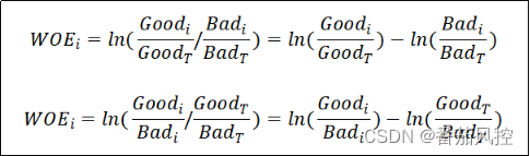

chart 1 WOE The principle formula

In view of the above WOE The formula , It can be described from two perspectives , The first formula can be understood as the difference between the good sample distribution and the bad sample distribution of each sub box , The second formula can be understood as the difference between the good / bad sample ratio of each sub box and the overall good / bad sample ratio . No matter from which derivation formula to understand , Its core ideas are consistent , That is to describe the difference between the distribution of good and bad samples in the box division of variables , And the final variable WOE The results are the same . Now through the actual example to verify the description , Suppose a characteristic variable is discretely divided into 10 Sub boxes （bin）, Count each score Good box 、 The number of bad samples is G_cnt、B_cnt, All samples are good 、 The number of bad samples is G_tot、B_tot, Through the above WOE The variables obtained by the two calculation formulas are divided into boxes WOE result , See the picture for details 2、 chart 3 Shown
​
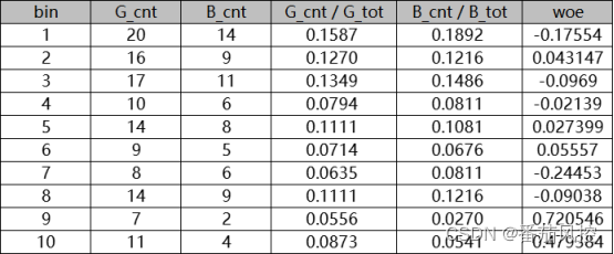
chart 2 WOE Principle logic 1

​
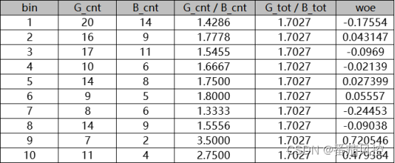
chart 3 WOE Principle logic 2

According to the distribution results in the above figure , Each sub box under two description modes WOE The results are consistent , It's just the difference in form . meanwhile , From the final result, we can see , With the difference between good and bad samples in each sub box interval of the variable ,WOE You can take a positive value 、 Negative or 0 All kinds of situations . What needs to be noted here is ,WOE Positive and negative value and size , That is what we need to focus on , And continuous sub box section WOE Changing relationships , It can reflect the differentiation ability and business attributes of variables to a large extent .
In an effort to 2 The variable of WOE Take the distribution result as an example , Separate boxes bin=1 Corresponding WOE The result is -0.17554, It shows that the performance of bad samples in this sub box interval is large , And WOE The greater the absolute value when it is negative , The worse the sample distribution is ; The opposite is true , Separate boxes bin=2 Corresponding WOE The result is 0.043147, It shows that the greater the performance of good samples in this sub box interval , And WOE The greater the absolute value when it is positive , The better the sample distribution is ; When the compartment WOE by 0 when , It shows that the performance of good and bad samples is quite .
Besides , It should be noted that ,WOE The positive and negative values represent the degree of good or bad samples , This rule is not absolute , The specific meaning depends on WOE Calculation formula settings . When the comparison relationship of sample distribution is like bad （Good/Bad） when , that WOE Timing means that the sample is good ; When the comparison relationship of sample distribution is bad, better （Bad/Good） when , that WOE Timing means that the sample is bad .

2、WOE Good and bad analysis
In order to further analyze the variable box interval WOE Business implications of , We aim at figure 2 Variable WOE The distribution results of , Further process other analysis indicators of each sub box interval ： Bad debt ratio badrate And information value IV, The calculation logic formula is shown in the figure 4 Shown .
​
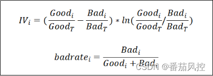
chart 4 IV And badrate Logic

From the above formula, we can see , Information value IV It can be further deduced as (Goodi/GoodT-Badi/BadT)*WOEi, Indicates the difference between the proportion of good and bad samples in each interval and WOE The product of . Besides , According to the variable IV The calculation formula of is easy to prove ,IV The value cannot be negative . Variable IV The value size is all sub box intervals IV Sum of values , When IV=0 Time indicates that the variable has no differentiation , And with the IV Increase of value , The stronger the ability of variables to distinguish good and bad samples , This principle is often used in the scene of feature variable screening , And it is an important step in the process of establishing models such as logistic regression . The indicator bad debt rate of the variable interval badrate It directly reflects the quality of the samples in the box division , That is, the proportion of bad samples in the total good and bad samples in the current interval , Through the comparative analysis with the bad debt rate of the overall sample , It can clearly compare the quality of samples in the box division . chart 2 The sample distribution corresponds to IV And badrate Indicator results , See the picture for details 5 Shown .
​
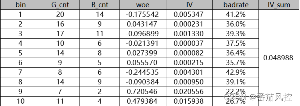
chart 5 IV And badrate result

​ From the results of the above figure , The bad debt rate of the whole sample is sum(G_cnt)/sum(G_cnt,B_cnt)=37%, Variable box interval WOE When it's negative , It shows that the bad degree of interval samples is relatively high （ Relative to the average quality of the overall sample ）, For example, the cartons in the figure bin=1、3、4、7、8 The interval of WOE All negative numbers , Corresponding bad debt rate badrate Are higher than the bad debt rate of the full sample （37%）; And the variable box interval WOE When it is a positive value , It shows that interval samples are relatively good , For example, the cartons in the figure bin=2、5、6、9、10 The interval of WOE All positive numbers. , Corresponding bad debt rate badrate Are lower than the bad debt rate of the full sample （37%）.
meanwhile , Regardless of the variable interval WOE Value is positive or negative , The greater the absolute value , It shows that the higher the degree of good or bad of the sample group , For example, sub box bin=1 And bin=3 Contrast ,WOE Respectively -0.175542、-0.096899, The absolute value of the former is larger than that of the latter , It indicates that the sample is more bad , Corresponding to bad debt rate badrate Respectively 41.2%、39.3% It directly verifies this Law . Another example is bin=9 And bin=10 Contrast ,WOE Respectively 0.020556、0.015938, First, a positive value indicates that the two interval samples are preferred to the overall sample distribution , Then the absolute value of the former is greater than the latter , It means that the sample is better , Let's look at the corresponding bad debt rate badrate Respectively 22.2%、26.7% , The former is better than the latter, which also verifies the analysis logic of the good or bad degree of the sample group .
This is through WOE Indicators to analyze the good or bad degree of the sample group in the variable interval , This has a good effect in evaluating the ability to distinguish variables , comparison badrate In terms of index analysis ,WOE Not only can the positive and negative relationship of the value reflect the good or bad bias of the interval sample compared with the overall sample , And it can further quantify the good or bad degree of the sample group according to the size relationship of the value . meanwhile , When WOE=0 It directly indicates that the good or bad degree of the interval is consistent with the average distribution of the overall sample , It is not necessary to predict the specific size of the bad debt rate of the full sample in advance , From these perspectives, we can comprehensively explain , Adopt variable WOE Value to evaluate the distribution characteristics of the box sample group has a good role . Besides , For continuous variables WOE Value distribution , It can be further used to analyze the monotonicity of variable differentiation , It provides a more convenient reference for the selection of modeling characteristic variables . chart 5 Variable WOE The distribution trend is displayed visually as shown in the figure 6 Shown , It can be seen from the final trend results , There is no obvious monotonicity in the differentiation of this variable , For the establishment of logical regression and other explanatory models , It is not convenient to adopt it into the model fitting variable pool
​
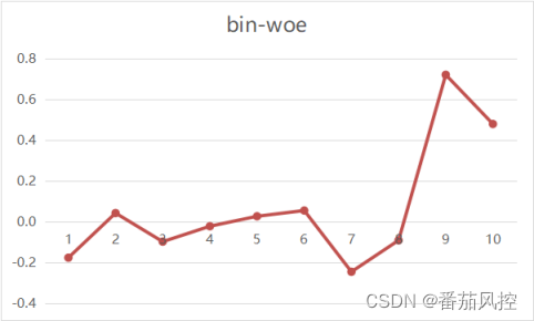
chart 6 Variable WOE Distribution trends

3、IV Ability to distinguish
In the figure 5 Of the index results , We get the interval of each sub box of variables synchronously IV Value size , You can see that ,WOE The greater the absolute value of ,IV The bigger the value is. , Describe from a business perspective , That is, the greater the difference between good and bad samples in the interval , The better the distinguishing ability of good and bad samples . For variable final IV value , Is composed of all intervals IV Sum the values to get , The larger the result is , Explain the distinguishing ability of variables （ Predictive power ） The stronger . For Graphs 5 Sample variables IV The value is 0.048988, How to evaluate in the actual business scenario , Or whether it can be selected as a modeling variable , There is no absolute standard , The details need to be determined comprehensively according to the sample situation and business needs . however , In general , Variable IV The value size represents the discrimination ability , A more general reference standard has been formed in the business , See the picture for details 7 Shown , It can be comprehensively applied in practice .
​
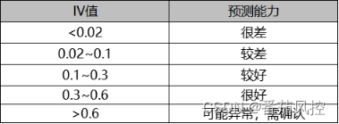
chart 7 Variable IV Evaluation criteria

4、WOE And IV example
Through the above introduction , We are familiar with variables as a whole WOE Calculation logic and analysis method , as well as WOE And IV The relationship between , Especially with WOE To analyze the good or bad degree of the variable box sample group , And evaluate the monotonic trend of variable differentiation ability , It is the key point that we must master in our daily data analysis work . Now let's combine a specific sample data , Implement variables through code WOE And IV Index output . Sample data （ front 10） Pictured 8 Shown , contain 6000 Samples and 6 A field , among ID Is the sample primary key ,X1~X4 Is the characteristic variable ,Y Is the target variable （ Value 0/1 They represent good and bad ）.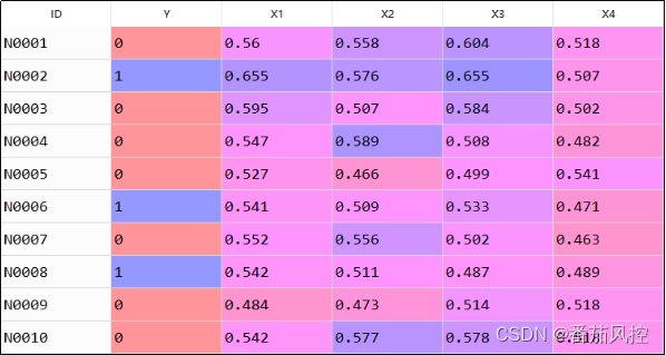

chart 8 Sample data

Now, the characteristic variable is divided into two parts by equal frequency X1~X4 Discrete as 10 box , And the number of good and bad sections 、 The proportion of good and bad 、 Bad debt ratio 、WOE、IV And other indicators are output uniformly , The specific implementation code is shown in figure 9 Shown .
​
chart 9 Feature sub box implementation

With characteristics X1 For example , The final packing result is shown in the figure 10 Shown , From the information in the table , Due to the equal frequency sub box method , The proportion of samples in each interval （percent） Both in 10% near . According to the variable woe The distribution shows , Variable X1 With the increase of the box division value , The difference between good and bad samples gradually develops in a good direction , Indicator bad debt rate badrate It can also verify this trend , And woe The monotonicity is also good , Pictured 11 Shown .
​
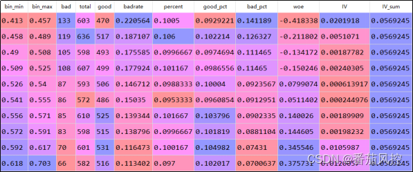
chart 10 Variable X1 Box division results

​
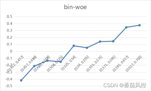
chart 11 Variable X1 monotonicity

In order to quickly convert all characteristic variables of sample data IV Value to output , You can use graphs 12 The loop code shown in , Variables of sample data X1~X4 Final IV The result is shown in Fig. 13 Shown . Of course , If you adjust the number of boxes , Or use other ways of dividing boxes （ Equidistant distribution box 、 Chi square sub box, etc ）, Variable box interval WOE Values and variables as a whole IV Values will change , The details need to be combined with the actual business scenarios , But no matter which kind of sub box method is adopted , For the features after the box WOE And IV The logic of analysis and its application are consistent .
​

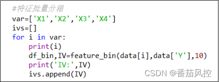
chart 12 Characteristic batch packing

​
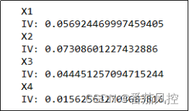
chart 13 Sample characteristics IV value

The above content is around the characteristics WOE Principle Logic and research ideas , It introduces WOE The application of indicators in analyzing the difference between good and bad samples in the actual scene , And combine variables IV Value describes the feature evaluation value of the two after feature discretization . In order to facilitate you to further understand and master the key points of this article , The sample data synchronized with the above example analysis and python Code , For your reference , For details, please move to the knowledge planet to view the relevant content .
​

…

~ Original article