Mobilenet series (4): mobilenetv3 network details

introduction

Nowadays, many lightweight networks often use MobileNetv3, This article will explain google Following MobileNetv2 Later proposed v3 edition .MobileNetv3 The paper ：Searching for MobileNetV3

according to MobileNetV3 The paper summary , The network has the following 3 Points that need your attention ：

• Updated Block(bneck), stay v3 This version of the original paper is called bneck, stay v2 edition Inverse residual structure A simple change has been made on the .
• Used NAS(Neural Architecture Search) Search parameters
• Redesigned the time-consuming structure : Author use NAS The network after searching , Next, the reasoning time of each layer of the network is analyzed , Some time-consuming layer structures are further optimized

MobileNetV3 Performance improvement

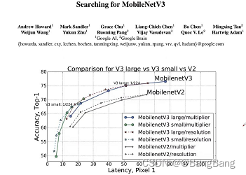
MobileNetV3-Large is 3.2% more accurate on ImageNet classification while reducing latency by 20% compared to MobileNetV2. MobileNetV3-Small is 6.6% more accurate compared to a MobileNetV2 model with comparable latency. MobileNetV3-Large detection is over 25% faster at roughly the same accuracy as MobileNetV2 on COCO detection. MobileNetV3-Large LRASPP is 34% faster than MobileNetV2 R-ASPP at similar accuracy for Cityscapes segmentation

• It can be seen that V3 Version of Large 1.0(V3-Large 1.0) Of Top-1 yes 75.2, about V2 1.0 its Top-1 yes 72, It's equivalent to a promotion 3.2%
• There is also a certain improvement in reasoning speed ,(V3-Large 1.0) stay P-1 The reasoning time on the mobile phone is 51ms, and V2 yes 64ms, Obviously V3 Than V2, Not only is it more accurate , And faster
• V3-Small Version of Top-1 yes 67.4, and V2 0.35 (0.35 Represents the magnification factor of the convolution kernel ) Of Top-1 Only 60.8, Improved accuracy 6.6%

Obviously V3 Version than V2 The version should be better

Network improvements

Updated Block

• Joined the SE modular （ Attention mechanism ）
• Updated activation function

MobieNetV2 Block

• First of all, it will pass a 1x1 Convolution layer to carry out dimension raising processing , After convolution, there will be BN and ReLU6 Activation function
• And then there was a 3x3 size DW Convolution , Convolution will still be followed by BN and ReLU6 Activation function
• The last accretion layer is 1x1 Convolution , Play the role of dimensionality reduction , Note that after convolution, only BN structure , Not used ReLU6 Activation function .

In addition, there is a shortcut branch in the network shotcut, Add our input characteristic matrix and output characteristic matrix on the same dimension . And only DW The convolution steps are 1, And input_channel==output_channel, Only then shotcut Connect

MobieNetV3 Block

What do you think , And MobieNetV2 Block It doesn't make any difference , The most obvious difference is that MobieNetV3 Block in SE modular （ Attention mechanism ）

SE modular

For the obtained characteristic matrix , For each channel Pool treatment , Next, through two Fully connected layer Get the output vector , The first fully connected layer , its Number of nodes in the full connection layer Is equal to the input characteristic matrix channel Of 1/4, The second fully connected layer channel Is related to our characteristic matrix channel Be consistent . After average pooling + Two fully connected layers , The output eigenvector can be understood as a pair of SE Each of the previous characteristic matrices channel A weight relation is analyzed , It thinks that the more important channel Will give a greater weight , For less important channel The dimension corresponds to a relatively small weight

As shown in the figure above ： Let's assume that the of our characteristic matrix channel by 2, Use Avg pooling For each channel To find an average , Because there are two channel, So get 2 Vectors of elements , Then it passes through two full connection layers in turn , first channel For the original channel Of 1/4, And it corresponds to relu Activation function . For the second fully connected layer, its channel And our characteristic matrix channel The dimensions are consistent , Note that the activation function used here makes h-sigmod, Then we get the sum characteristic matrix channel A vector of the same size , Each element corresponds to each channel Of The weight . For example, the first element is 0.5, take 0.5 And the first of the characteristic matrix channel Multiply the elements of , Get a new one channel data .

In addition, the network has updated the activation function

Corresponds to NL It is a nonlinear activation function , The activation functions used in different layers are different , There is no explicit activation function here , It is marked with a NL, Pay attention to the last layer 1x1 There is no nonlinear activation function used in the convolution of , Using a linear activation function .

MobieNetV3 Block and MobieNetV2 Block The structure is basically the same , Mainly increased SE structure , The activation function is updated

Redesign the time-consuming layer structure

stay Original thesis It mainly talks about two parts ：

• Reduce the number of convolutions of the first convolution layer (32 -> 16)
  stay v1,v2 The number of convolution kernels in the first layer of the version is 32 Of , stay v3 In this version, we only use 16 individual
  
  In the original paper , The author said that the convolution kernel Filter Number from 32 Turn into 16 after , Its accuracy is the same as 32 It's the same , Since the accuracy has no effect , With less convolution kernel, the amount of computation becomes smaller . I'm saving roughly 2ms Operation time of
• Streamlining Last Stage
  In the use of NAS The last part of the searched network structure , be called Original last Stage, Its network structure is as follows ：
  
  The network is mainly generated by stacking convolution , The author found this in the course of use Original Last Stage It is a time-consuming part , The author has simplified the structure , Came up with a Efficient Last Stage

Efficient Last Stage Compared with the previous Original Last Stage, A lot less convolution , The author found that the accuracy of the updated network is almost unchanged , But it saves 7ms Execution time of . this 7ms Occupy the reasoning 11% Time for , Therefore use Efficient Last Stage after , It is quite obvious for us to improve our speed .

Redesign the activation function

Before that v2 We basically use ReLU6 Activation function , Now the commonly used activation function is swish Activation function .
$$swithx=x.\sigma (x)$$
among $\sigma$ The calculation formula of is as follows ：
$$\sigma (x)=\frac{1}{1+e^{-x}}$$
Use switch After activating the function , It can really improve the accuracy of the network , But there are 2 A question ：

• Calculation 、 Derivation is complicated
• Unfriendly to the quantification process ( For mobile devices , Basically, it will be quantified for acceleration )

Because of the problem , The author put forward that h-switch Activation function , Talking about h-switch Before activating the function, let's talk about h-sigmoid Activation function

h-sigmoid The activation function is in relu6 Activate the function to modify ：
$$RELU6(x)=min(max(x,0),6)$$
$$h-sigmoid=\frac{ReLU6(x+3)}{6}$$

As you can see from the diagram h-sigmoid And sigmoid The activation function is close to , So in many scenarios h-sigmoid Activate the function to replace our sigmoid Activation function . therefore h-switch in $\sigma$ Replace with h-sigmoid after , The form of the function is as follows :
$$h-switch[x]=x\frac{ReLU6(x+3)}{6}$$

As shown in the right part of the above figure , yes switch and h-switch Comparison of activation functions , Obviously the two curves are very similar , So using h-switch To replace switch The activation function is great .

In the original paper , The author said that h-switch Replace switch, take h-sigmoid Replace sigmoid, For the reasoning process of the network , It is helpful in reasoning speed , It is also very friendly to the quantification process .

MobieNetV3-Large Version of the network structure

Simply look at the meanings of the parameters in the following table ：

• input Input layer characteristic matrix shape
• operator It means operation , For the first convolution layer conv2d; there
• #out Of the output characteristic matrix channel, We said it was v3 The first convolution kernel in this version uses 16 Convolution kernels
• there NL Represents the activation function , among HS It stands for hard switch Activation function ,RE It stands for ReLU Activation function ;
• there s Representative DW Convolution step ;
• there beneck Corresponding to the structure in the figure below ;
• exp size Represents the first convolution of ascending dimensions , How many dimensions are we going to raise ,exp size How many? , We'll use the first floor 1x1 How many dimensions does convolution rise to .
• SE: Indicates whether the attention mechanism is used , As long as the form is awarded √ The corresponding bneck Structure uses our attention mechanism , Yes, No √ You won't use the attention mechanism
• NBN The last two convolutions operator Tips NBN, Indicates that these two convolutions do not use BN structure , The last two convolutions are equivalent to the function of full connection
• Be careful ： first bneck structure , There is something special here , its exp size And the input characteristic matrix channel It's the same , Originally bneck The first convolution in plays the role of L d The role of , But there is no upgrade here . So in the process of implementation , first bneck There is no structure 1x1 Convolutional , It is a direct analysis of our characteristic matrix DW Convolution processing

bneck

• First, through 1x1 Convolution is carried out to increase the dimension to exp size, adopt DW The dimension of convolution will not change , Similarly passed SE after channel Will it change . Finally through 1x1 Convolution for dimensionality reduction . After the dimension reduction channel Corresponding to #out The value given .
• about shortcut Shortcut Branch , Must be DW The convolution steps are 1, And bneck Of input_channel=output_channel Only then shortcut Connect

Through this table, we can build MobilenetV3 Network structure

about MobileNetV3-Small Network structure , as follows , I won't talk about it here , It is basically consistent with what I said .

MobileNetV3-Small