当前位置:网站首页>Medical image segmentation
Medical image segmentation
2022-07-06 18:35:00 【HammerHe】
1.U-Net
After reading several posts, this one is more posted !!
Introduction : Common image formats for medical images :
(1)DICOM
(2)MHD/RAW
(3)NRRD
1.1 U-Net The architecture of
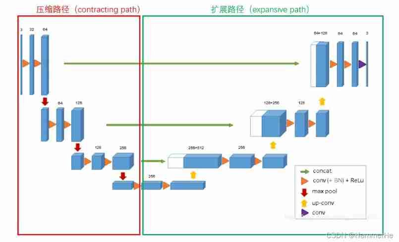
U-Net Of U The shape structure is shown in the figure below . Network is a classical full convolution network ( That is, there is no full connection operation in the network ). Belong to FCN Improved type of . In a sense U-Net The whole process is encoding and decoding (encoder-decoder) The process of , Information compression is coding , Information extraction is decoding , Such as images , Text , Video compression and decompression .
The input to the network is a 572x572 The edge of the image is mirrored (input image tile)
The network path is divided into two parts :
(1) Compress path (contracting path)
On the left side of the network ( Red dotted line ) It's made up of convolution and Max Pooling A series of downsampling operations , This part is called compression path in this paper (contracting path).
The compression path is created by 4 individual block form , Every block Used 3 Two efficient convolutions and 1 individual Max Pooling Downsampling , After each downsampling Feature Map Multiply by 2, So there's the Feature Map Change in size . Finally, we get the size of 16x16 Of Feature Map.
(2) Extension path (expansive path)
The extended path is designed to improve the resolution of the output . For positioning , The sampling output is combined with the high-resolution features of the whole model . then , The sequence convolution layer aims to produce a more accurate output based on this information .
The right side of the network ( Dotted green line ) It's called extension path in the paper (expansive path). By the same 4 individual block form , Every block Before you start, deconvolute Feature Map Multiply the size of 2, At the same time, reduce the number by half ( The last layer is slightly different ), And then with the left symmetric compression path Feature Map Merge , Because of the difference between the left compressed path and the right extended path Feature Map It's not the same size ,U-Net By compressing the path Feature Map Crop to the same size as the extended path Feature Map To normalize ( That is, the dotted line on the left in the figure below ). The convolution operation of extended path still uses effective convolution operation , resulting Feature Map Its size is 388x388 . Because this task is a binary task , So the network has two outputs Feature Map.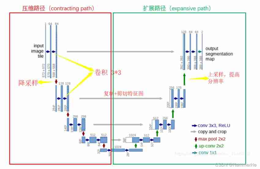
1.2 Preprocessing ( Increase contrast 、 Denoise )
stay U-Net The denoising method used in image preprocessing is image denoising based on curvature drive
In the field of image denoising , Due to Gaussian low-pass filtering on all high-frequency components of the image Without distinction Ground weakening , Thus, the edge is blurred while the noise is removed .
Isoilluminance lines formed by objects in natural images ( Including the edges ) It should be a smooth enough curve , That is, the absolute value of the curvature of these isoilluminance lines should be small enough . When the image is polluted by noise , The random fluctuation of the local gray value of the image leads to the irregular oscillation of the isoilluminance line , Form isoilluminance lines with large local curvature , Therefore, all high-frequency components of the image conform to the change of curvature To differentiate Ground weakening , Thus, the effect of image denoising will be very good . According to this principle , Image denoising can be carried out .
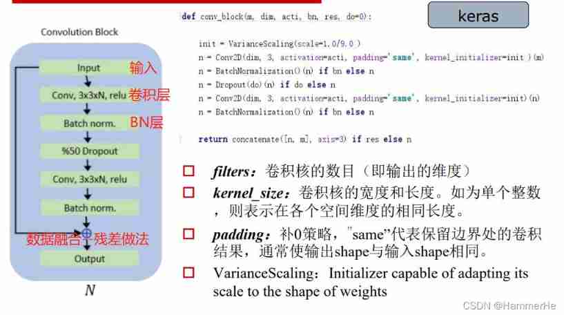
1.2 Convolution block model
1.3 Objective function -Dice coefficient
Dice Distance is used to measure the similarity between two sets , Because strings can be understood as a set , therefore Dice The distance can be used to calculate the similarity of two strings and the difference of graphic mask area .
Dice The coefficients are defined as follows :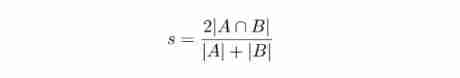 Dice The value range of the coefficient is 0 To 1. In form ,Dice Sum of coefficients Jaccard Index (A hand over B Divide A and B) No big difference , It can be converted to each other .
About the loss function : The same in U-NET It uses the loss function and FCN Similar are loss functions with boundary weights , But combined Dice Loss calculation , That is, the sum of standard binary cross entropy Dice Function of loss calculation :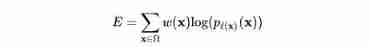
1.4 Methods of image enhancement
There are only a few dozen original data sets , Far from enough to train 7 layer U-Net This is of great significance 5000W+ A deep network of parameters . I used keras Self contained image data enhancement technology , Translate the original data 、 rotate 、 Twist and other operations ( Including the corresponding annotation data ) .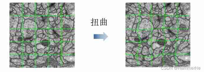
For translation and rotation, we mainly use Affine transformation .
For twist operation , An important way is Elastic deformation ( Introduction post ):
Elastic deformation :
On the original lattice , Superimpose positive and negative random distances to form “ Interpolation position ” matrix , Then calculate the gray level at each interpolation position , Form a new lattice [Simard,2003], To realize the distortion and deformation inside the image . The specific theoretical steps can be seen in the introduction post .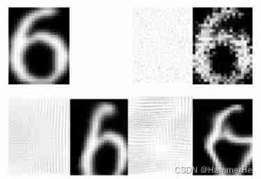
1.5 U-net Problem legacy
(1) The top section and bottom section of tissues and organs are too different from the middle section to be easily identified ;(2) There are large appearance variations between different scanned images, which are difficult to identify ;
(3) Artifact and distortion caused by magnetic field inhomogeneity , It is difficult to identify .
2. 3D U-Net
Why 3D U-net?
Biomedical imaging (biomedical images) A lot of times Lump Of , That is to say, it consists of many slices (slice) The existence of a whole picture . If it is to use 2D Image processing model (U- Net) To deal with 3D It's not impossible , But there will be a problem , I have to make a picture of biomedical images slice One slice Grouped ( Including training data and labeled data ) Send in the designed model for training , And a large number of 3 Annotation of dimensional images is tedious and inefficient , Because adjacent slices display almost the same information . And in this case, there will be an efficiency problem , Therefore, it is very complicated to deal with block graphs , And the way of data preprocessing is relatively cumbersome (tedious).
therefore 3D -Net The model is to solve the problem of efficiency , And for the cutting of block graph, only some slices in the data are required to be marked .
3D U-net Two methods of :
There are two ways :
(1) One is semi-automatic setting , Train on a sparsely labeled dataset and predict other unlabeled places on this dataset ;
(2) Train on multiple sparse labeled datasets , Then generalize to new data .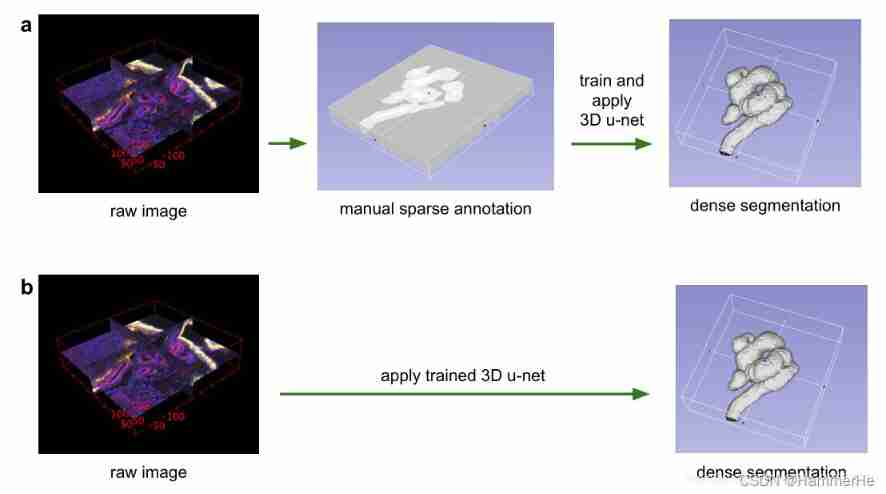 The above figure well expresses the two methods in the paper :
(a) Use a few slices to make a complete dense prediction ( Stereo segmentation );
(b) Train the model on the labeled data set , Then apply it to the new unmarked data to make intensive prediction directly .
2.1 3D U-Net Network structure
3D Unet Network structure and 2D Unet The network is very similar , Just put all 2D All operations are replaced by 3D operation . namely 3D U-NET The Internet is a way to 3D Data as input , And use the corresponding operation to process the data , Include 3D Convolution 、3D Maximum pool and 3D Upward convolution .
Suppose the size of the input data is a1 × a2 × a3, The number of channels is c, The filter size is f, That is, the filter dimension is f × f × f × c, The number of filters is n. Then the final output of three-dimensional convolution is ( a1 - f + 1 ) × ( a2 - f + 1 ) × ( a3 - f + 1 ) × n .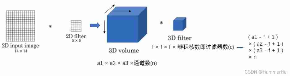 In addition, the difference lies in the timing of doubling the number of channels and deconvolution operation . stay 2D Unet in , The time to double the number of channels is the first convolution after down sampling ; And in the 3D Unet in , The doubling of the number of channels occurs in the convolution before down sampling or up sampling . For deconvolution , The difference is whether the number of channels is halved ,2D Unet Halve the number of channels in , and 3D Unet The number of channels in the does not change .
Besides ,3D Unet Also used batch normalization To accelerate convergence and avoid the bottleneck of network structure .
3D U-net The specific structure of is details :
And two-dimensional U-NET equally , It has compressed paths ( Analysis path ) And extension path ( Synthesis path ), The architecture has a total of 19069955 Parameters
 The details are introduced below :
(1) In the compressed path , Each layer contains two 3×3×3 A convolution , Each one follows one (Relu), Then on each dimension 2×2×2 The maximum pool merges two steps .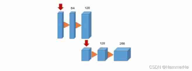 (2) In the extended path , Each layer consists of 2×2×2 The upper convolution of , The step size on each dimension is 2, Then there are two 3×3×3 A convolution , And then there was Relu.
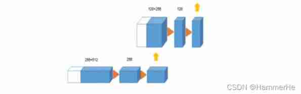 (3) From the equal resolution layer in the compression path shortcut Connections provide basic high-resolution features of extended paths .
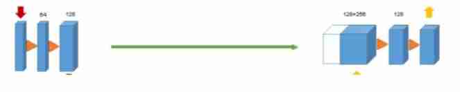 (4) In the last layer ,1×1×1 Convolution reduces the number of output channels , The number of labels is 3.
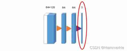
You can see the overall structure and details with U-Net similar , Here are the main points :
(1) And U-Net Input comparison , The input here is a stereoscopic image (132×132×116), And is 3 individual channel.
(2)ReLU I added BN layer , To accelerate convergence and avoid the bottleneck of network structure .
(3) By doubling before maximizing pooling doubling Number of channels channels To avoid bottlenecks.
3. V-Net
Vnet Yes, also for 3D The model proposed by the image .V-Net That's right U-net A deformation of . At this time, the data set can be directly used 3D Data sets . The final output is also single channel 3D data . It can deal with the serious imbalance between the number of foreground and background voxels 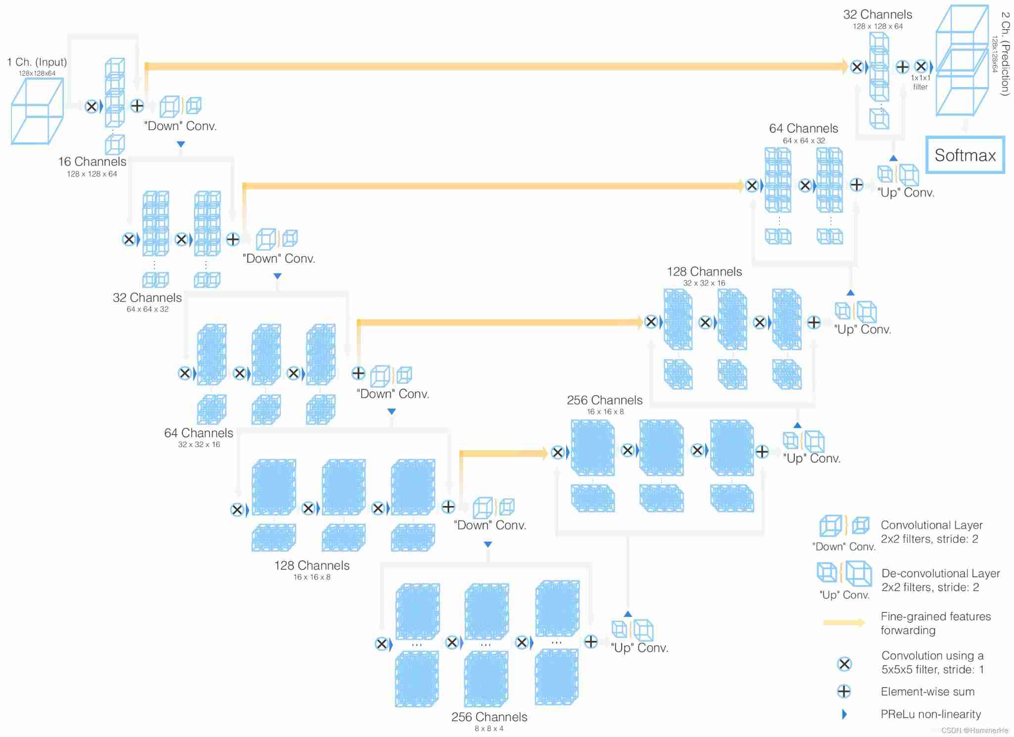 Network structure details and innovations :
1. Introduce residuals
What needs special explanation here , It's also Vnet and Unet The biggest difference , It's in every stage in ,Vnet Adopted ResNet Short circuit connection mode ( Grey route ),. Equivalent to the Unet Introduction in ResBlock. This is a Vnet The biggest improvement . It is similar to using the pycnocline connection .
The residual link in the horizontal direction is borrowed Unet Stack from compressed path feature map Methods , So as to supplement the method of loss information ( Yellow line ). That is, send the bottom feature of the zoom in end to the corresponding position of the zoom in end to help reconstruct a high-quality image , And accelerate the convergence of the model .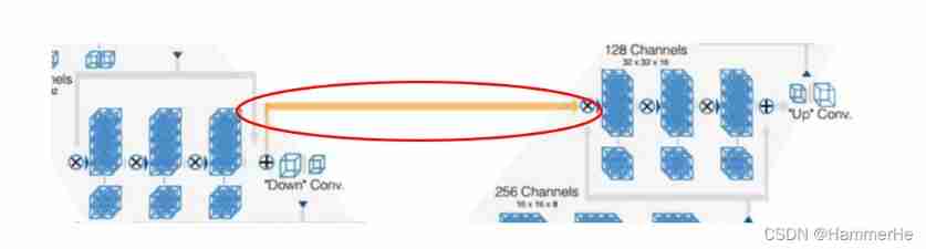
2. be based on Dice A new objective function of coefficients
Again based on Dice coefficient , But don't just ReLU 了 , The objective function used is PReLU, It refers to the addition of parameter correction ReLU, The parameter α Need training and learning .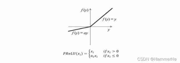
3. The convolution layer replaces the pooling layer of up sampling and down sampling
Every stage The convolution kernel used at the end of is 2x2x2,stride by 2 Convolution of , Feature size reduced by half . That is, use the appropriate stride ( Greater than 1) Of 3D Convolution to reduce the size of the data .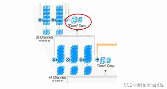 This process is more intuitively shown as follows , The first half is convolution instead of pooling to reduce the size :
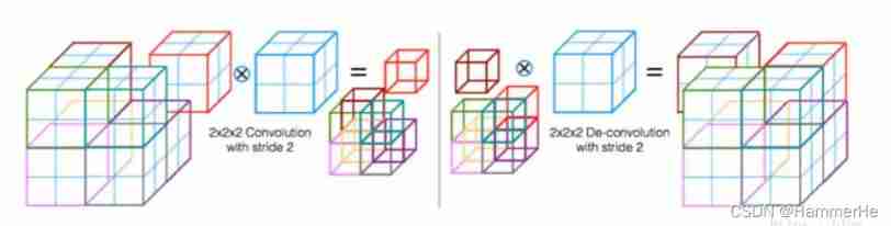
4. End treatment
Add a at the end of the network 111 Convolution of , Processing into data of the same size as the input , And then one after another softmax most , stay softmax after , The output consists of a probability plot of the background and foreground .
With high probability (>0.5) Voxels belong to foreground , Not the background , Considered to be part of an organ .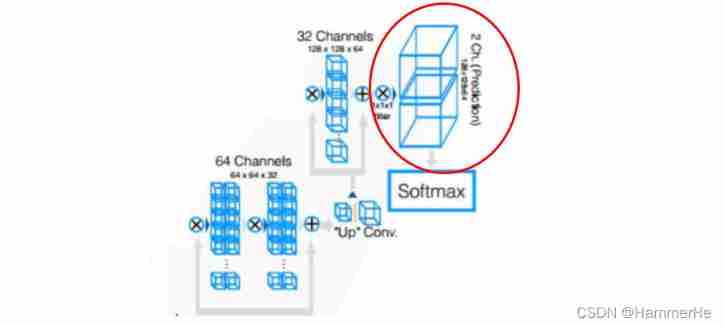
5. Improve the data expansion method
(1) utilize 2x2x2 Grid control points and B-spline The dense deformation field is obtained to randomly deform the image .
(2) Histogram matching
4.DenseNet( In order to elicit FC-DenseNet)
One about DenseNet Features and details of a relatively complete interpretation post
First, make sure that DenseNet Is a new connection mode , and ResNet as well as GoogleNet It's almost the same use .
In previous years, convolutional neural network is the direction to improve the effect :
(1) Or deep , Deepen the number of network layers , such as ResNet, It solves the problem of gradient disappearing when the network is deep
(2) Either wide , Widen the network structure , such as GoogleNet Of Inception
DenseNet Away from deepening the number of network layers (ResNet) And widened network structure (Inception) To improve network performance
From features feature From the perspective of , Through feature reuse and bypass (Bypass) Set up , It not only greatly reduces the amount of network parameters , To a certain extent, it alleviated gradient vanishing Problem generation . The assumption of combining information flow and feature reuse
4.1 DenseNet Some of the advantages of :
(1) To reduce the vanishing-gradient( The gradient disappears )
(2) Strengthened feature The transitivity of , Make more effective use of feature
(3) To some extent, it reduces the number of parameters
(4) Emphasize parameter validity , High parameter efficiency
(5) Implicit deep supervision ,short paths;
(6) Over fitting , Especially when training data is scarce
4.2 DenseNet Network structure
actually DenseNet The core of the network is to ensure the maximum information transmission between the middle layers of the network , Connect all layers directly !
Let's put one first dense block Structure diagram .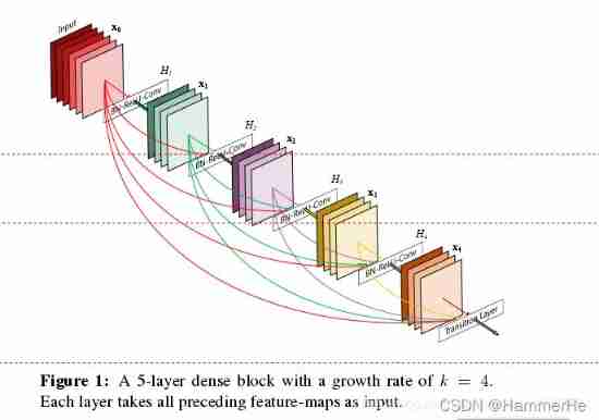
In the traditional convolution neural network , If you have L layer , Then there will be L A connection , But in DenseNet in , There will be L(L+1)/2 A connection . In short , The input of each layer comes from the output of all previous layers . Here's the picture :x0 yes input,H1 The input is x0(input),H2 The input is x0 and x1(x1 yes H1 Output ), And so on :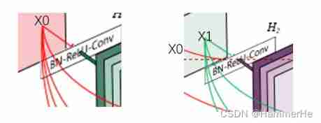
Specific network structure diagram :
This Table1 It's the structure of the whole network . In this table k=32,k=48 Medium k yes growth rate, Represent each dense block Output of each layer in feature map Number .
In order to avoid the network becoming very wide , The authors use smaller ones k, such as 32 such , The author's experiments also show that Small k Can have a better effect .
according to dense block The design of the , The next few layers can get input from all the previous layers , therefore concat After the input channel It's still bigger .
(1)bottleneck layer: At every dense block Of 33 Convolution is preceded by a 11 Convolution operation of , That's what's called bottleneck layer
The goal is to reduce input feature map Number , It can reduce the dimension and the amount of calculation , It can also integrate the characteristics of each channel .
(2)Translation layer: To further compress the parameters , In every two dense block And then there's an increase in 11 Convolution operation of . This is the addition of this Translation layer, This layer of 11 The output of convolution channel The default is input channel Half way through .
about DenseNet-C This network is added Translation layer
about DenseNet-BC The network , It means that there is already bottleneck layer, And then there is Translation layer.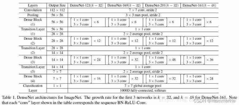
5.FC-DenseNet
On this network and U-Net In fact, there is not much difference in essence , It is the combination of compressed path and expanded path , But in FC-DenseNet Used in Dense Block and Transition Up To replace the up sampling operation in the full convolution network , among Transition Up Use transpose convolution to upsample the characteristic graph , Then with the characteristics of layer jumping Concatenation Become new together Dense Block The input of . Use this layer hopping solution Dense Block The problem of feature loss in .
5.1 FC-DenseNet Network structure
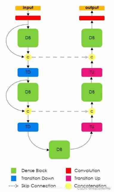
As shown in the figure above :
stay FC-DenseNet The right side uses Dense block and transition up Replace FC Convolution operation of up sampling .Transition up Use transpose convolution to upsample the characteristic graph , It is connected in series with the features from the layer hopping , Generate a new dense block The input of .
But this will lead to a linear increase in the number of characteristic graphs , To solve this problem ,dense block The input of is not connected in series with its output . At the same time, the structure of layer hopping is introduced to solve the problem before dense block The problem of feature loss
So what is dense block The input of is not connected in series with its output ? Following pair dense block Module expansion introduction :
(1)Dense Block modular
dense block The structure is as follows: , Make the first layer input x0 Yes m A feature map , The first layer outputs x1 Yes k A feature map , this k A characteristic graph and m Characteristic graphs are connected in series , As input to the second layer , repeat n Time ;
The first N Layer of layer After layer output and before layer Output merge , share N×k A feature map . And input m Not in series with the output .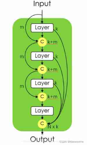
(2) Specific network structure 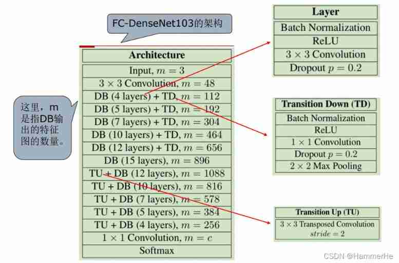
边栏推荐
猜你喜欢
随机推荐
287. Find duplicates
Cobra quick start - designed for command line programs
Bonecp uses data sources
Cobra 快速入门 - 专为命令行程序而生
递归的方式
Numerical analysis: least squares and ridge regression (pytoch Implementation)
【Swoole系列2.1】先把Swoole跑起来
2022-2024年CIFAR Azrieli全球学者名单公布,18位青年学者加入6个研究项目
2022 Summer Project Training (II)
徐翔妻子应莹回应“股评”:自己写的!
This article discusses the memory layout of objects in the JVM, as well as the principle and application of memory alignment and compression pointer
测试123
2019阿里集群数据集使用总结
2022 Summer Project Training (I)
传输层 拥塞控制-慢开始和拥塞避免 快重传 快恢复
使用cpolar建立一个商业网站(1)
Stm32+mfrc522 completes IC card number reading, password modification, data reading and writing
win10系统下插入U盘有声音提示却不显示盘符
巨杉数据库首批入选金融信创解决方案!
C language college laboratory reservation registration system