当前位置:网站首页>Deep Learning (3) Classification Theory Part
Deep Learning (3) Classification Theory Part
2022-08-04 02:32:00 【Ali forever】
分类 理论部分
前言
This article will revolve around how to realize the classification model with adjustable parameters in this area for this
一、反向传播
在深度学习神经网络中,Optimization generally using the gradient descent method to adjust our parameters,But because the network layer of the neural network is too complex,Derivation is very difficult,Therefore, there is a very convenient method in the computer to reduce the computational complexity.
1.chain rule math formula
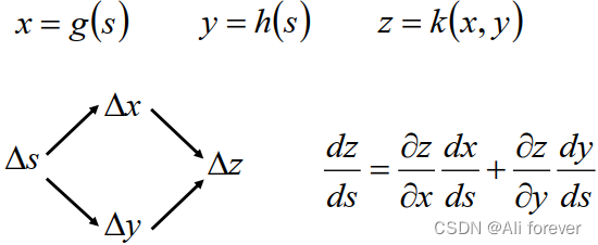
2.正向传播的过程

L ( θ ) = ∑ n = 1 N ( y n − y ^ n ) = ∑ n = 1 N C n ( θ ) L(\theta)=\sum_{n=1}^{N}(y^n-\hat{y}^n)=\sum_{n=1}^{N}C^n(\theta) L(θ)=n=1∑N(yn−y^n)=n=1∑NCn(θ)
∂ L ( θ ) ∂ w = ∑ n = 1 N ∂ C n ( θ ) ∂ w \frac{\partial L(\theta)}{\partial w}=\sum_{n=1}^{N}\frac{\partial C^n(\theta)}{\partial w} ∂w∂L(θ)=n=1∑N∂w∂Cn(θ)
Here we pick one ofC对权重w求偏导,根据链式法则We can take the partial derivative split into:
∂ C ∂ w = ∂ z ∂ w ∗ ∂ C ∂ z \frac{\partial C}{\partial w}=\frac{\partial z}{\partial w}*\frac{\partial C}{\partial z} ∂w∂C=∂w∂z∗∂z∂C
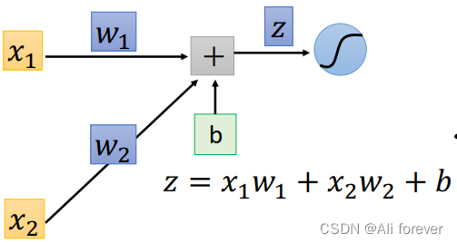
可以知道 ∂ z ∂ w 1 \frac{\partial z}{\partial w_1} ∂w1∂z= x 1 x_1 x1, ∂ z ∂ w 2 \frac{\partial z}{\partial w_2} ∂w2∂z= x 2 x_2 x2,这个过程我们叫做正向传播(Forward Pass),So our question focuses on how to solve ∂ C ∂ z \frac{\partial C}{\partial z} ∂z∂C中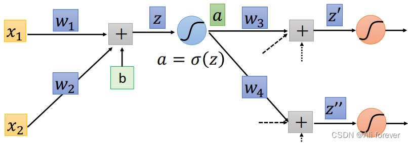
我们可以看到zThrough an activation function can be called a new resulta,This is we can also through the chain rule to split:
∂ C ∂ z = ∂ a ∂ z ∗ ∂ C ∂ a \frac{\partial C}{\partial z}=\frac{\partial a}{\partial z}*\frac{\partial C}{\partial a} ∂z∂C=∂z∂a∗∂a∂C
可以知道 ∂ a ∂ z \frac{\partial a}{\partial z} ∂z∂a= σ ′ ( z ) \sigma'(z) σ′(z),那么如何求解 ∂ C ∂ a \frac{\partial C}{\partial a} ∂a∂Cbecomes a very difficult thing,Because according to the chain rule
∂ C ∂ a = ∂ z ′ ∂ a ∗ ∂ C ∂ z ′ + ∂ z ′ ′ ∂ a ∗ ∂ C ∂ z ′ ′ \frac{\partial C}{\partial a}=\frac{\partial z'}{\partial a}*\frac{\partial C}{\partial z'}+\frac{\partial z''}{\partial a}*\frac{\partial C}{\partial z''} ∂a∂C=∂a∂z′∗∂z′∂C+∂a∂z′′∗∂z′′∂C
At this time how we will continue to derive formula is complicated,And if the later matures more and more,will grow exponentially,So we don't do forward propagation anymore,接下来我们将进行反向传播(Backpropagation)
3.反向传播的过程
Suppose we spread through positive all the weight and the activation function of the derivative was calculated,then the result will be: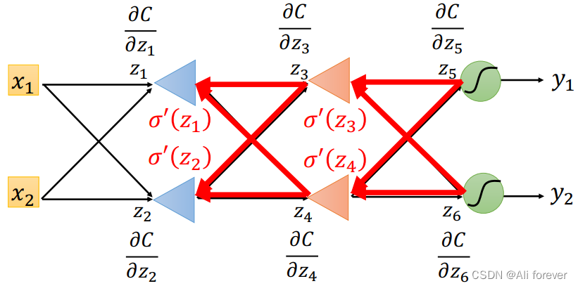
For the last output layer:
∂ C ∂ z 5 = ∂ y 1 ∂ z 5 ∗ ∂ C ∂ y 1 \frac{\partial C}{\partial z_5}=\frac{\partial y_1}{\partial z_5}*\frac{\partial C}{\partial y_1} ∂z5∂C=∂z5∂y1∗∂y1∂C ∂ C ∂ z 6 = ∂ y 2 ∂ z 6 ∗ ∂ C ∂ y 2 \frac{\partial C}{\partial z_6}=\frac{\partial y_2}{\partial z_6}*\frac{\partial C}{\partial y_2} ∂z6∂C=∂z6∂y2∗∂y2∂CBoth of these results are easy to obtain,After getting these two results,We can then continue to calculate the parameters that were missing from our previous forward pass,在这里我们举个简单的例子:
∂ C ∂ a ( z 4 ) = ∂ z 5 ∂ a ( z 4 ) ∗ ∂ C ∂ z 5 + ∂ z 6 ∂ a ( z 4 ) ∗ ∂ C ∂ z 6 \frac{\partial C}{\partial a(z_4)}=\frac{\partial z_5}{\partial a(z_4)}*\frac{\partial C}{\partial z_5}+\frac{\partial z_6}{\partial a(z_4)}*\frac{\partial C}{\partial z_6} ∂a(z4)∂C=∂a(z4)∂z5∗∂z5∂C+∂a(z4)∂z6∗∂z6∂C
After this calculation,You can fill in all the missing items in forward propagation..
二、Preliminary knowledge of classification(Classification)
在前面的内容里,We introduce how to do regression,But not all problems are regression problems,We will introduce another problem below,也就是分类问题
1.Similarities and differences between classification and regression
The similarities of regression and classification:都是监督学习,both make predictions about the input,然后得到预测值
The difference between classification and regression is in the following aspects:
输出不同
The categorical output is a discrete variable,是一种定性输出,Determine the type of object,The regression output is a continuous variable.,是一种定量输出,得到输出值目的不同
The purpose of classification is mainly to find a decision plane,On the whole plane to classify the data,The purpose of regression is to find the best fit,通过回归算法得到是一个最优拟合线,这个线条可以最好的接近数据集中的各个点.结果不同
Classification results are only right or wrong,The regression result is based on whether it is closer to the true value as the standard,rather than simply judging right or wrong.使用场景不同
Classification can be used for confirmation of handwritten signatures,Confirmation of face recognition,Confirmation of illness, etc..while regression can be used for similar house prices,The weather forecast.
2.Regression is used as the classification?
This idea stems from the fact that a predicted value is obtained by regression,By judging which classification value is close to,determine which classification value,这种想法是错误的.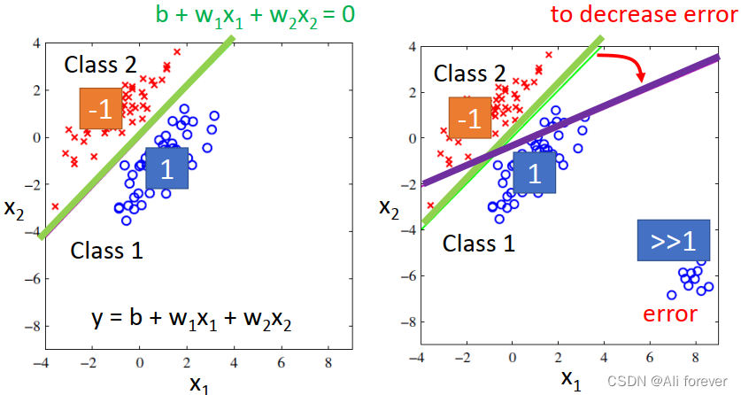
在这一幅图中,We can see that there are far greater1的值,According to our theory above,这些远大于1points will be judged as1,But in fact they are the wrong point,This leads to a misjudgment.
3.贝叶斯公式
We take a simple example to smoke ball as an introduction:
先验概率与后验概率:
先验概率:假设抽取Box1的概率是 2 3 \frac{2}{3} 32,抽取Box2的概率是 1 3 \frac{1}{3} 31,即P( B 1 B_1 B1)= 2 3 \frac{2}{3} 32,P( B 2 B_2 B2)= 1 3 \frac{1}{3} 31,These two probabilities are the prior probabilities.
后验概率:when we know from B 1 B_1 B1For the ball inside,The probability of drawing blue isP( B l u e ∣ B 1 Blue|B_1 Blue∣B1)= 4 5 \frac{4}{5} 54,The probability of drawing green isP( G r e e n ∣ B 1 Green|B_1 Green∣B1)= 1 5 \frac{1}{5} 51
Conditional probability formula and total probability formula:
条件概率公式: P ( A B ) = P ( A ∣ B ) ∗ P ( B ) = P ( B ∣ A ) ∗ P ( A ) P(AB)=P(A|B)*P(B)=P(B|A)*P(A) P(AB)=P(A∣B)∗P(B)=P(B∣A)∗P(A)其中P(AB)是A与B的联合概率
全概率公式:如果事件 A 1 A_1 A1、 A 2 A_2 A2… … A i A_i Ai构成一个完备事件组,即它们两两互不相容,其和为全集,则有:
P ( B ) = ∑ n = 1 N P ( A i ) P ( B ∣ A i ) P(B)=\sum_{n=1}^{N}P(A_i)P(B|A_i) P(B)=n=1∑NP(Ai)P(B∣Ai)
贝叶斯公式
P ( B 1 ∣ B l u e ) = P ( B 1 , B l u e ) P ( B l u e ) = P ( B l u e ∣ B 1 ) ∗ P ( B 1 ) P ( B l u e ∣ B 1 ) ∗ P ( B 1 ) + P ( B l u e ∣ B 2 ) ∗ P ( B 2 ) P(B_1|Blue)=\frac{P(B_1,Blue)}{P(Blue)}=\frac{P(Blue|B_1)*P(B_1)}{P(Blue|B_1)*P(B_1)+P(Blue|B_2)*P(B_2)} P(B1∣Blue)=P(Blue)P(B1,Blue)=P(Blue∣B1)∗P(B1)+P(Blue∣B2)∗P(B2)P(Blue∣B1)∗P(B1)
三、生成模型与判别模型
Supervised learning is generally divided into generative models and discriminative models,So what's the difference between the two??
1.生成模型(generative model)
源头导向型,关注数据时如何生成的,然后再对一个信号进行分类.(信号输入时,生成模型判断哪个类别最有可能产生这个信号,则这个信号就属于哪个类别.
We use a simple example to illustrate:
There's a bunch of balls now,Two kinds of color information known as the green and yellow,There are only two colors,这里,The color of the ball isy(目标变量),The position on the coordinate axis is the featureX.我们想要知道,If a location on the axisxput in a new ball,What color is this club?
We can easily calculatey的先验概率P(y),And the posterior probabilityP(x|y=green),
P(x|y=yellow)Can estimate by training,get a result like the following: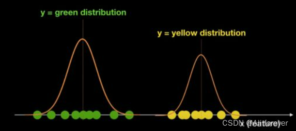
Then according to the conditional probability formula we can calculate the joint probabilityP(x,y=green),P(x,y=yellow)
If it is a binary classification problem, you can get the final result by judging which probability is greater.
2.判别模型(Discriminative Model)
结果导向型,关注类别之间的差别,并不关心样本的数据时怎么生成的,根据样本之间的“分界线"来简单对给定的样本进行分类.
We also use the above example to illustrate: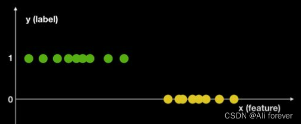
First we put this figure into this,Then in the next step we can calculateP(Y|X),By calculation we can get a line through some algorithm,来进行判别.
3.The difference between the generated model and the discriminant model
- 特点
A generative model is a statistical representation of the distribution of data,Can reflect the similarity of similar data.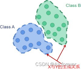
The discriminative model is to find the optimal segmentation surface for different classifications,反映数据的差异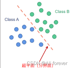
Generative models can be transformed into discriminative models by Bayesian formula,But the discriminative model cannot be converted into a generative model - 优缺点
Advantages of generative models:
- Can be used when data is incomplete
- 收敛速度快,Faster convergence to the true model
- 存在隐变量时,still usable,Carry more information than discriminative models
- Less chance of overfitting,The research question more flexible
The advantages of discriminant model: - 结果很直观,Can see the difference between one class and other classes at a glance
- Apply to more categories
- 判别模型更加简单,Convenient for learning and training
生成模型的缺点: - Requires a large amount of data as a training set,Not friendly with little data
- The distribution function is vulnerable to the entry of some outliers
- Features that are very similar,容易产生假阳性
Disadvantages of discriminative models: - 黑盒操作,The relationship between the variables is not clear,不可视
- 常见模型
生成模型:朴素贝叶斯分类器,马尔科夫模型,高斯混合模型,Limit Pullman Machines
判别模型:逻辑回归,决策树,k近邻,线性回归,SVM,boosting - 常见用途
生成模型:NLP,医疗诊断
判别模型:Image text classification,时间序列检测
四、高斯分布(Gaussian Distribution)With the maximum likelihood function(Maximum Likelihood)
1.Why use a Gaussian distribution?
Because many events in nature are independent random events,This random variable is close to a Gaussian distribution,So this has been assumed to be an independent random event,If there is a serious correlation, we generally do not use.
其次,In the case of known mean and variance of gaussian distribution entropy is the largest of all distribution,When the data distribution is unknown, the model with the largest entropy is usually selected
2.Two-dimensional Gaussian distribution formula
f μ , Σ ( x ) = 1 ( 2 π ) 2 D 1 ∣ Σ ∣ 1 2 e x p { − 1 2 ( x − μ ) T Σ − 1 ( x − μ ) } f_{\mu,\Sigma}(x)=\frac{1}{(2\pi)^{2D}}\frac{1}{|\Sigma|^{\frac{1}{2}}}exp\{-\frac{1}{2}(x-\mu)^T{\Sigma}^{-1}(x-\mu)\} fμ,Σ(x)=(2π)2D1∣Σ∣211exp{ −21(x−μ)TΣ−1(x−μ)}
We should know that the most important thing in the Gaussian distribution formula is the mean μ \mu μWith the covariance matrix Σ \Sigma Σ,These two parameters determine the overall probability density distribution,We will use maximum likelihood estimation to calculate them
3.最大似然估计
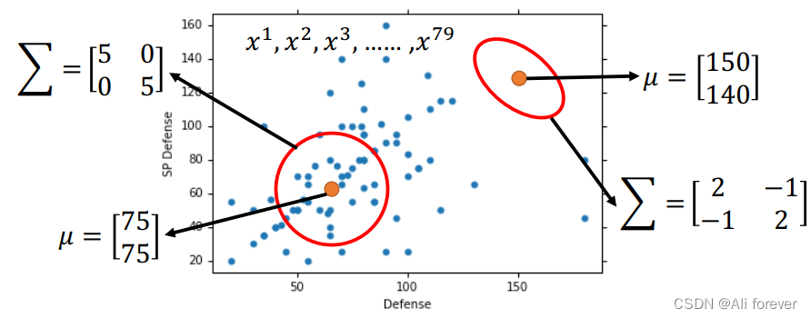
Since each point selected here will have a different mean μ \mu μWith the covariance matrix Σ \Sigma Σ,Then we can multiply their probability density functions together,得到:
L ( μ , Σ ) = f μ , Σ ( x 1 ) f μ , Σ ( x 2 ) . . . . . . f μ , Σ ( x n ) L(\mu,\Sigma)=f_{\mu,\Sigma}(x^1)f_{\mu,\Sigma}(x^2)......f_{\mu,\Sigma}(x^n) L(μ,Σ)=fμ,Σ(x1)fμ,Σ(x2)......fμ,Σ(xn)
Then our goal is to get
μ ∗ , Σ ∗ = arg max μ ∗ , Σ ∗ L ( μ , Σ ) \mu^*,\Sigma^*=\arg\max_{\mu^*,\Sigma^*} L(\mu,\Sigma) μ∗,Σ∗=argμ∗,Σ∗maxL(μ,Σ)
最后计算得到:
μ ∗ = 1 N ∑ n = 1 N x n , Σ ∗ = 1 N ∑ n = 1 N ( x n − μ ∗ ) ( x n − μ ∗ ) T \mu^*=\frac{1}{N}\sum_{n=1}^{N}x^n,\Sigma^*=\frac{1}{N}\sum_{n=1}^{N}(x^n-\mu^*)(x^n-\mu^*)^T μ∗=N1n=1∑Nxn,Σ∗=N1n=1∑N(xn−μ∗)(xn−μ∗)T
Once all of the optimal solution of parameters calculated,can be substituted into the original Gaussian distribution,Since the posterior probability follows a Gaussian distribution,we can substitute data,calculate the result.
4.Gaussian distribution optimization
Since the covariance matrix has a lot to do with the number of eigenvalues of the input,If there are too many eigenvalues,A larger covariance matrix can have a big impact on the results,So we can consider sharing a covariance matrix,thereby reducing errors.
weighted average below,其中 α \alpha α为 μ 1 \mu_1 μ1in all μ \mu μ中的占比.
Σ = α Σ 1 + ( 1 − α ) Σ 2 \Sigma = \alpha\Sigma_1+(1-\alpha)\Sigma_2 Σ=αΣ1+(1−α)Σ2
when taking the same Σ \Sigma Σ的时候,We will find that his decomposition frontier is a linear model.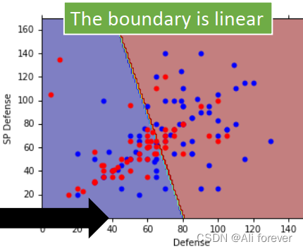
这是因为,Our posterior probability eventually translates to P ( C 1 ∣ x ) = σ ( w x + b ) P(C_1|x)=\sigma(wx+b) P(C1∣x)=σ(wx+b),But this is essentially findingw跟b的值,If you use generative models, you will waste time,Next, there will be another way to quickly find this result.
五、逻辑回归(Logistic Regression)
It was introduced when the discriminant model was introduced above.,逻辑回归是一种判别模型,Mainly solve the problem of binary classification
1.函数集(Function Set)
z = ∑ i w i x i + b z=\sum_iw_ix_i+b z=i∑wixi+b
P w , b ( C 1 ∣ x ) = σ ( z ) = σ ( ∑ i w i x i + b ) P_{w,b}(C_1|x)=\sigma(z)=\sigma(\sum_iw_ix_i+b) Pw,b(C1∣x)=σ(z)=σ(i∑wixi+b)
2.The quality of the evaluation function(Goodness of a Function)

We can see so many characteristics of the corresponding category respectively,Next we want to calculate for aw跟ba probability density function of
L ( w , b ) = f w , b ( x 1 ) f w , b ( x 2 ) ( 1 − f w , b ( x 3 ) ) . . . . . . f w , b ( x N ) L(w,b)=f_{w,b}(x^1)f_{w,b}(x^2)(1-f_{w,b}(x^3))......f_{w,b}(x^N) L(w,b)=fw,b(x1)fw,b(x2)(1−fw,b(x3))......fw,b(xN)
In the same way, we call the maximum likelihood estimation to find the bestw与b值,Generally, in order to reduce the amount of calculation,We will take the logarithm,This converts the product into the sum of the terms
w ∗ , b ∗ = arg max w ∗ , b ∗ L ( w , b ) = arg min w ∗ , b ∗ − ln L ( w , b ) w^*,b^*=\arg\max_{w^*,b^*} L(w,b)=\arg\min_{w^*,b^*}-\ln L(w,b) w∗,b∗=argw∗,b∗maxL(w,b)=argw∗,b∗min−lnL(w,b)
Next we will construct交叉熵(cross entropy)
H ( p , q ) = − ∑ x p ( x ) ln ( q ( x ) ) H(p,q)=-\sum_xp(x)\ln(q(x)) H(p,q)=−x∑p(x)ln(q(x))
在这里p(x)refers to the actual distribution,q(x)refers to the distribution of maximum likelihood estimates,So each item can become like this:
− ln f w , b ( x 1 ) = − ( y ^ 1 ln f w , b ( x 1 ) + ( 1 − y ^ 1 ) ln ( 1 − f w , b ( x 1 ) ) ) -\ln f_{w,b}(x^1)=-(\hat{y}^1\ln f_{w,b}(x^1)+(1-\hat{y}^1)\ln (1-f_{w,b}(x^1))) −lnfw,b(x1)=−(y^1lnfw,b(x1)+(1−y^1)ln(1−fw,b(x1)))
The total cross-entropy function becomes:
− ln L ( w , b ) = − ∑ n ( y ^ n ln f w , b ( x n ) + ( 1 − y ^ n ) ln ( 1 − f w , b ( x n ) ) ) -\ln L(w,b)=-\sum_n(\hat{y}^n\ln f_{w,b}(x^n)+(1-\hat{y}^n)\ln (1-f_{w,b}(x^n))) −lnL(w,b)=−n∑(y^nlnfw,b(xn)+(1−y^n)ln(1−fw,b(xn)))
Cross-entropy represents how close two distributions are,If the same two distribution,则交叉熵为0,If the two distributions are very different,then the cross entropy is large.
3.找到最佳的函数(Find the best function)
− ln L ( w , b ) ∂ w i = − ∑ n ( y ^ n ln f w , b ( x n ) ∂ w i + ( 1 − y ^ n ) ln ( 1 − f w , b ( x n ) ) ∂ w i ) \frac{-\ln L(w,b)}{\partial w_i}=-\sum_n(\frac{\hat{y}^n\ln f_{w,b}(x^n)}{\partial w_i}+\frac{(1-\hat{y}^n)\ln (1-f_{w,b}(x^n))}{\partial w_i}) ∂wi−lnL(w,b)=−n∑(∂wiy^nlnfw,b(xn)+∂wi(1−y^n)ln(1−fw,b(xn)))
∂ ln f w , b ( x n ) ∂ w i = ∂ z ∂ w i ∂ ln f w , b ( x n ) ∂ z = x i ∗ 1 σ ( z ) ∗ σ ( z ) ∗ ( 1 − σ ( z ) ) \frac{\partial \ln f_{w,b}(x^n)}{\partial w_i}=\frac{\partial z}{\partial w_i}\frac{\partial\ln f_{w,b}(x^n)}{\partial z}=x_i*\frac{1}{\sigma(z)}*\sigma(z)*(1-\sigma(z)) ∂wi∂lnfw,b(xn)=∂wi∂z∂z∂lnfw,b(xn)=xi∗σ(z)1∗σ(z)∗(1−σ(z))
∂ ln ( 1 − f w , b ( x n ) ) ∂ w i = ∂ z ∂ w i ∂ ln ( 1 − f w , b ( x n ) ) ∂ z = x i ∗ 1 1 − σ ( z ) ∗ ( 1 − σ ( z ) ) ∗ ( σ ( z ) ) \frac{\partial \ln(1- f_{w,b}(x^n))}{\partial w_i}=\frac{\partial z}{\partial w_i}\frac{\partial\ln (1-f_{w,b}(x^n))}{\partial z}=x_i*\frac{1}{1-\sigma(z)}*(1-\sigma(z))*(\sigma(z)) ∂wi∂ln(1−fw,b(xn))=∂wi∂z∂z∂ln(1−fw,b(xn))=xi∗1−σ(z)1∗(1−σ(z))∗(σ(z))
∂ − ln L ( w , b ) ∂ w i = − ∑ n y ^ n ∗ x i n ∗ ( 1 − σ ( z ) ) − ( 1 − y ^ n ) ∗ x i n ∗ σ ( z ) = − ∑ n ( y ^ n − σ ( z ) ) ∗ x i n \begin{split} \frac{\partial -\ln L(w,b)}{\partial w_i}&=-\sum_n\hat{y}^n*x_i^n*(1-\sigma(z))-(1-\hat{y}^n)*x_i^n*\sigma(z)\\ &=-\sum_n(\hat{y}^n-\sigma(z))*x_i^n \end{split} ∂wi∂−lnL(w,b)=−n∑y^n∗xin∗(1−σ(z))−(1−y^n)∗xin∗σ(z)=−n∑(y^n−σ(z))∗xin
Finally get the update function:
w i = w i − η ∑ n ( y ^ n − σ ( z ) ) ∗ x i n w_i=w_i-\eta\sum_n(\hat{y}^n-\sigma(z))*x_i^n wi=wi−ηn∑(y^n−σ(z))∗xin
Comparing update functions for linear and logistic regression,You will find they look exactly the same,just logistic regression y ^ n \hat{y}^n y^n只能取值0或者1,Linear regression can take many different values.
4.The loss of the logistic regression function
在前面我们说到,The loss function selected by logistic regression is cross entropy,instead of the mean square error we mentioned in linear regression,这是为什么呢?
这是因为当 σ ( z ) \sigma(z) σ(z)=0或者1时,整个loss function的结果都为0,That is to say, both cases will be found guilty of convergence,false positive problem,这是不可取的,So we won't use mean square error in logistic regression.
总结
This paper presents the theoretical part of the classification,Hope you can get what you want from it,A mind map is attached below to help memory.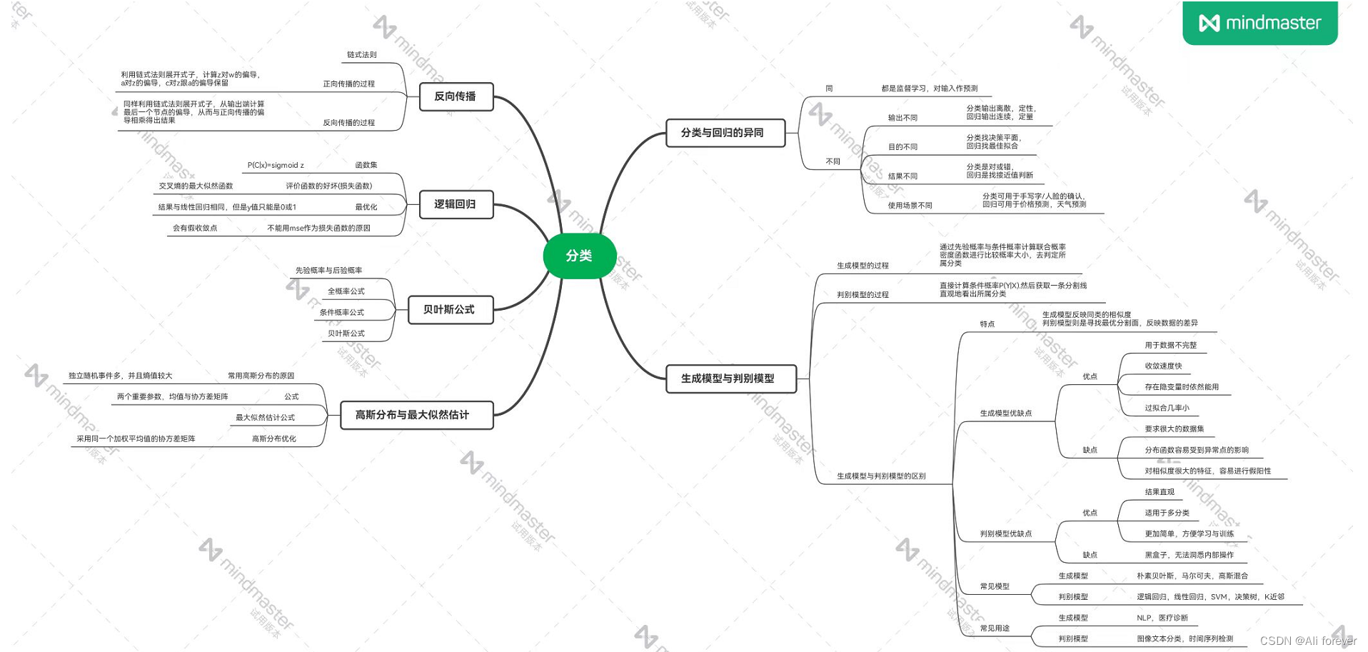
边栏推荐
猜你喜欢
cdh6.x 集成spark-sql

持续投入商品研发,叮咚买菜赢在了供应链投入上

出海季,互联网出海锦囊之本地化
Example 041: Methods and variables of a class

MallBook 助力SKT思珂特教育集团,立足变化,拥抱敏捷交易
编写 BOLL 心得体会
单片机C语言->的用法,和意思

lombok注解@RequiredArgsConstructor的使用

Continuing to invest in product research and development, Dingdong Maicai wins in supply chain investment
云开发旅游打卡广场微信小程序源码(含视频教程)
随机推荐
Instance, 038: the sum of the diagonal matrix
共n级台阶,每次可以上1级或2级台阶,有多少种上法?
2022.8.3-----leetcode.899
STM8S-----选项字节
Example: 036 is a prime number
参加Oracle OCP和MySQL OCP考试的学员怎样在VUE预约考试
【学习笔记之菜Dog学C】动态内存管理
Multithreading JUC Learning Chapter 1 Steps to Create Multithreading
深度学习(三)分类 理论部分
DDTL: Domain Transfer Learning at a Distance
Variable string
Example 041: Methods and variables of a class
Development of Taurus. MVC WebAPI introductory tutorial 1: download environment configuration and operation framework (including series directory).
工程制图复习题(带答案)
实例040:逆序列表
idea中diagram使用
实例041:类的方法与变量
Oracle迁移到瀚高之后,空值问题处理
flask框架初学-06-对数据库的增删改查
Kubernetes:(十一)KubeSphere的介绍和安装(华丽的篇章)
