当前位置:网站首页>Notes of training courses selected by Massey school
Notes of training courses selected by Massey school
2022-07-07 00:27:00 【Evergreen AAS】
Multivariate statistical analysis
Clustering analysis
characteristic :
- I don't know the number and structure of categories in advance ;
- The data to be analyzed is the similarity or dissimilarity between objects ( distance );
- Put objects close together .
classification
- According to different classification objects, it can be divided into
- Q Type clustering : Cluster the samples
- R Type clustering : Cluster variables
- According to the clustering method, it is mainly divided into
- Systematic clustering
- Dynamic clustering
distance
Minikowski distance :
d(x,y) = [\sum\limits_{k=1}^p|x_{k} - y_{k}|^{m}]^{\frac{1}{m}}, x,y by p Virial vector
- m = 1 when , Is absolute distance
- m = 2 when , For Euclidean distance
- m = \infty, For Chebyshev distance , namely \mathop{max}\limits_{1\le k \le p}|x_{k} - y_{k}|
Mahalanobis distance ( Commonly used in cluster analysis )
d(x,y) = \sqrt{(x - y)^{T} \sum\nolimits^{-1} (x - y)}
among x, y For coming from p Dimensional population Z Sample observations of ,Σ by Z The covariance matrix of , In the actual Σ Often do not know , It is often necessary to estimate with sample covariance . Markov distance is invariant to all linear transformations , Therefore, it is not affected by dimensions .
R sentence :
dist(x,method=“euclidean”, diag=FALSE, upper=FALSE, p=2)
- method: The way to calculate the distance
- “euclidean”: Euclidean distance
- “maximum”: Chebyshev distance
- “manhattan”: Absolute distance
- “minkowski”: Minkowski distance ,p yes Minkowski Order of distance
- diag=TRUE: Output the distance on the diagonal
- upper=TRUE: Output the value of the upper triangular matrix ( The default value is only output The value of trigonometric matrix )
python sentence :
import rpy2.robjects as robjects

x = [1, 2, 6, 8, 11]
r = robjects.r
res = r.dist(x)
print(res)
#    1  2  3  4
# 2  1
# 3  5  4
# 4  7  6  2
# 5 10  9  5  3
import rpy2
import rpy2.robjects.numpy2ri

R = rpy2.robjects.r
r_code = """
x<-c(1,2,6,8,11)
y<-dist(x)
print(y)
"""
R(r_code)
- notes : I use rpy2 It's hard to realize this feeling . It may not be possible to learn from python call R Language , Direct use recommended R Language
Standardized treatment
When the measured values of indicators differ greatly , The data should be standardized first , Then use the standardized data to calculate the distance .
General standardized transformation
X_{ij}^{*} = \frac{X_{ij} - \overline{X}_{j}}{S_{j}}
i=1,2,…n It means the first one i Samples ,j=1,2,…p Represents the... Of the sample j Indicators , Each sample has p Two observation indicators . It's No j Sample mean of indicators
Range standardization transformation
X_{ij}^{*} = \frac{X_{ij} - \overline{X}_{j}}{R_{j}} \\ among ,R_{j} = \mathop{\max}\limits_{1\le k \le n}X_{kj} - \mathop{\max}\limits_{1 \le k \le n}X_{kj}
Range normalization transformation
X_{ij}^{*} = \frac{X_{ij} - \mathop{\min}\limits_{1\le k\le n} X_{kj}}{R_{j}}
Program statement
Centralization and standardization of data
R sentence
scale(X,center = True, scale = True)
X: Sample data matrix ,center = TURE Means to make centralized transformation of data ,scale=TRUE It means to make standardized changes to the data
python sentence
import rpy2
import numpy
import rpy2.robjects.numpy2ri

rpy2.robjects.numpy2ri.activate()

R = rpy2.robjects.r
x = numpy.array([[1.0, 2.0], [3.0, 1.0]])
res = R.scale(x, center=True, scale=True)
print(res)
The data is subject to extreme standardization
x <- data.frame(
    points = c(99, 97, 104, 79, 84, 88, 91, 99),
    rebounds = c(34, 40, 41, 38, 29, 30, 22, 25),
    blocks = c(12, 8, 8, 7, 8, 11, 6, 7)
)
# apply() Function must be applied to dataframe or matrix
center <- sweep(x, 2, apply(x, 2, mean))
R <- apply(x, 2, max) - apply(x, 2, min)
x_star <- sweep(center, 2, R, "/")
#  if x_star<-sweep(center, 2, sd(x), "/"),  Then we get ( Ordinary ) Standardized transformed data ;
print(x_star)
sweep(x, MARGIN, STATS, FUN=”-“, …)
- x: Array or matrix ;MARGIN: Operation area , The matrix 1 Said line ,2 The column ;
- STATS It's statistics ,apply(x, 2, mean) Represents the mean value of each column ;
- FUN Represents the operation of a function , The default value is subtraction .
Similarity coefficient
Calculate the correlation coefficient between different indicators of the sample , It is suitable for clustering variables .
Systematic clustering
Cluster analysis is the most commonly used
The basic idea
- (1) Depending on each sample ( Or variable ) Self becoming , Specify the distance between classes ( Or the coefficient of similarity );
- (2) Take the most similar sample ( Or variable ) Gather into small categories , Then aggregate the aggregated subclasses according to similarity ;
- (3) Finally, all subclasses are aggregated into a large class , Thus, we can get a pedigree relationship gathered according to the size of similarity
3. According to different definitions of distance, it can be divided into
- (1) The shortest distance method : The distance between classes is defined as the distance between the nearest samples in the two classes ;
- (2) The longest distance method : The distance between classes is defined as the distance between the farthest samples in the two classes ;
- (3) Class average method : The distance between classes is defined as the average of the distance between two samples in two classes ;
Program
 x<-c(1,2,6,8,11);
dim(x)<-c(5,1);
d<-dist(x) # Generate distance structure
hc1<-hclust(d, "single"); hc2<-hclust(d, "complete")
hc3<-hclust(d, "median"); hc4<-hclust(d, "mcquitty") # Generate systematic clustering
opar <- par(mfrow = c(2, 2))
plot(hc1,hang=-1); plot(hc2,hang=-1)
plot(hc3,hang=-1); plot(hc4,hang=-1)
par(opar)#   Draw all tree structure diagrams , With 2*2 The form of is drawn on a picture
hclust(): Calculate the systematic clustering plot(): Draw a tree diagram of systematic clustering hclust(d, method = “complete”) d:dist Distance structure , method: The method of systematic clustering ( The default is the longest distance method ), The parameters are : (1)“single”: The shortest distance method (2)“complete”: The longest distance method (3)“average”: Class average method …… plot(x, labels = NULL, hang = 0.1, main = “Cluster Dendrogram”, sb = NULL, xlab = NULL, ylab =”Height”, …)
x: hclust() The object generated by the function hang: Indicate the positions of various types in the tree , Taking a negative value means that the classes in the tree are drawn from the bottom main: Drawing name
Dynamic clustering
System clustering : Once the class is formed, it will not change ; Dynamic clustering : Stepwise clustering
The basic idea
First, roughly classify , Then modify the unreasonable classification according to some optimal principle , Until the score is reasonable , Form the final classification result .
Program
kmeans(x, centers, iter.max=10, nstart=1, algorithm*=c(“Hartigan-Wong”, “Lloyd”, “MacQueen”))
- x It is a matrix or data frame composed of data ,
- centers Is the number of clusters or the center of the initial class ,
- iter.max Is the maximum number of iterations ( The maximum value is 10),
- nstart Is the number of random sets ,
- algorithm It is a dynamic clustering algorithm .
X<-data.frame(
   x1=c(2959.19, 2459.77, 1495.63, 1046.33, 1303.97, 1730.84, 1561.86, 1410.11, 3712.31, 2207.58, 2629.16, 1844.78, 2709.46, 1563.78, 1675.75, 1427.65, 1783.43, 1942.23, 3055.17, 2033.87, 2057.86, 2303.29, 1974.28, 1673.82, 2194.25, 2646.61, 1472.95, 1525.57, 1654.69, 1375.46, 1608.82),
   x2=c(730.79, 495.47, 515.90, 477.77, 524.29, 553.90, 492.42, 510.71, 550.74, 449.37, 557.32, 430.29, 428.11, 303.65, 613.32, 431.79, 511.88, 512.27, 353.23, 300.82, 186.44, 589.99, 507.76, 437.75, 537.01, 839.70, 390.89, 472.98, 437.77, 480.99, 536.05),
   x3=c(749.41, 697.33, 362.37, 290.15, 254.83, 246.91, 200.49, 211.88, 893.37, 572.40, 689.73, 271.28, 334.12, 233.81, 550.71, 288.55, 282.84, 401.39, 564.56, 338.65, 202.72, 516.21, 344.79, 461.61, 369.07, 204.44, 447.95, 328.90, 258.78, 273.84, 432.46),
   x4=c(513.34, 302.87, 285.32, 208.57, 192.17, 279.81, 218.36, 277.11, 346.93, 211.92, 435.69, 126.33, 160.77, 107.90, 219.79, 208.14, 201.01, 206.06, 356.27, 157.78, 171.79, 236.55, 203.21, 153.32, 249.54, 209.11, 259.51, 219.86, 303.00, 317.32, 235.82),
   x5=c(467.87, 284.19, 272.95, 201.50, 249.81, 239.18, 220.69, 224.65, 527.00, 302.09, 514.66, 250.56, 405.14, 209.70,272.59, 217.00, 237.60, 321.29, 811.88, 329.06, 329.65, 403.92, 240.24, 254.66, 290.84, 379.30, 230.61, 206.65, 244.93, 251.08, 250.28),
   x6=c(1141.82, 735.97, 540.58, 414.72, 463.09, 445.20, 459.62, 376.82, 1034.98, 585.23, 795.87, 513.18, 461.67, 393.99, 599.43, 337.76, 617.74, 697.22, 873.06, 621.74, 477.17, 730.05, 575.10, 445.59, 561.91, 371.04, 490.90, 449.69, 479.53, 424.75, 541.30),
   x7=c(478.42, 570.84, 364.91, 281.84, 287.87, 330.24, 360.48, 317.61, 720.33, 429.77, 575.76, 314.00, 535.13, 509.39, 371.62, 421.31, 523.52, 492.60, 1082.82, 587.02, 312.93,438.41, 430.36, 346.11, 407.70, 269.59, 469.10, 249.66, 288.56, 228.73, 344.85),
   x8=c(457.64, 305.08, 188.63, 212.10, 192.96, 163.86, 147.76, 152.85, 462.03, 252.54, 323.36, 151.39, 232.29, 160.12, 211.84, 165.32, 182.52, 226.45, 420.81, 218.27, 279.19, 225.80, 223.46, 191.48, 330.95, 389.33, 191.34, 228.19, 236.51, 195.93, 214.40),
   row.names = c(" Beijing ", " tianjin ", " hebei ", " shanxi ", " Inner Mongolia ", " liaoning ", " Ji Lin ", " heilongjiang ", " Shanghai ", " jiangsu ", " Zhejiang ", " anhui ", " fujian ", " jiangxi ", " Shandong ",  " Henan ", " hubei ", " hunan ", " guangdong ", " guangxi ", " hainan ", " Chongqing ", " sichuan ", " guizhou ", " yunnan ", " Tibet ", " shaanxi ", " gansu ", " qinghai ", " ningxia ", " xinjiang ")
)

kmeans(scale(X),5)


K-means clustering with 5 clusters of sizes 10, 7, 3, 7, 4


Clustering vector:
   Beijing     tianjin     hebei     shanxi   Inner Mongolia     liaoning     Ji Lin   heilongjiang     Shanghai     jiangsu
     5      4      3      3      3      3      3      3      5      4
   Zhejiang     anhui     fujian     jiangxi     Shandong     Henan     hubei     hunan     guangdong     guangxi
     5      1      2      1      4      1      1      4      5      2
   hainan     Chongqing     sichuan     guizhou     yunnan     Tibet     shaanxi     gansu     qinghai     ningxia
     2      4      1      1      4      4      1      3      3      3
   xinjiang
     3
Principal component analysis
The basic idea
The importance of variables in practical problems is different , And there is a certain correlation between many variables . These variables are transformed through this correlation , Use a small number of new variables to reflect most of the information provided by the original variables , Simplify the original problem . That is, data dimensionality reduction
Principal component analysis is a statistical method for processing high-dimensional data under this dimensionality reduction idea .
The basic method
By properly constructing the linear combination of original variables , Generate a new list of unrelated variables , Select a few new variables and make them contain as much information as the original variables , Thus, a few new variables are used to replace the original variables , To analyze the original problem .
The variable contains “ Information ” The size of is usually measured by the variance of the variable or the sample variance .
Such as constant a,Var(a) = 0 , We go through a, I can only know a This constant , It contains little information .
Definition of principal component
set up X = (X_{1}, X_{2},……,X_{p})^{T} For practical problems involved p A vector of random variables , remember X The mean of \mu, The covariance matrix is \sum.
Consider linear combinations
\left\{ \begin{aligned} Y_{1} & = & a_{1}^{T}X \\ . \\ . \\ Y_{p} & = & a_{p}^{T}X \\ \end{aligned} \right.
………………………………………………………………………………………………………
warning: Just write the code
Program
Find the eigenvalue and eigenvector of the matrix
a <- c(1, -2, 0, -2, 5, 0, 0, 0, 2)
#  By vector a Construction one 3 Columns of the matrix , byrow=T The data representing the generated matrix is placed in rows ;
b <- matrix(data = a, ncol = 3, byrow = T)
c <- eigen(b) #  seek b Eigenvalues and eigenvectors of
Linear model
1. The relationship between variables is generally divided into two categories
- Completely certain relationship , It can be expressed as a function analytic expression
- Uncertain relationship , Also known as correlation
2. The main content of regression analysis
- Through observation or processing of experimental data , Find out the quantitative mathematical expression of the correlation coefficient between variables — Empirical formula , That is, parameter estimation , And determine the specific form of empirical regression equation
- Test whether the established empirical regression equation is reasonable
- Use a reasonable regression equation for random variables Y Predict and control .
边栏推荐
- Leecode brush questions record sword finger offer 11 Rotate the minimum number of the array
- C语言输入/输出流和文件操作【二】
- Business process testing based on functional testing
- 沉浸式投影在线下展示中的三大应用特点
- Typescript incremental compilation
- uniapp中redirectTo和navigateTo的区别
- 从外企离开,我才知道什么叫尊重跟合规…
- [boutique] Pinia Persistence Based on the plug-in Pinia plugin persist
- 微信小程序uploadfile服务器,微信小程序之wx.uploadFile[通俗易懂]
- A way of writing SQL, update when matching, or insert
猜你喜欢
如何判断一个数组中的元素包含一个对象的所有属性值
The way of intelligent operation and maintenance application, bid farewell to the crisis of enterprise digital transformation
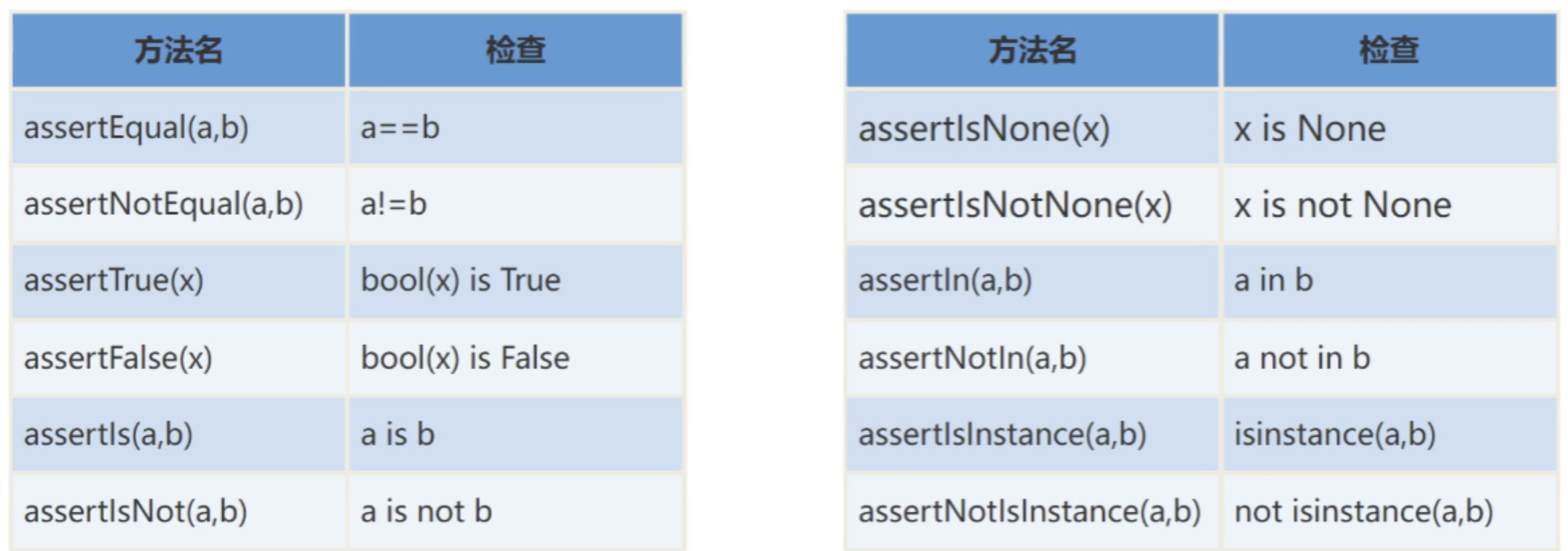
【自动化测试框架】关于unittest你需要知道的事
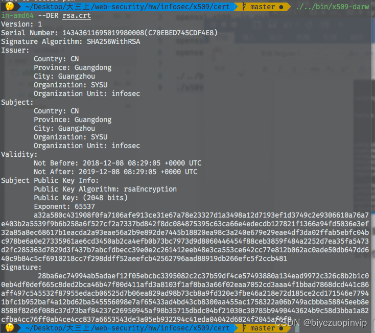
基於GO語言實現的X.509證書
2022/2/10 summary

48 page digital government smart government all in one solution
![[2022 the finest in the whole network] how to test the interface test generally? Process and steps of interface test](/img/8d/b59cf466031f36eb50d4d06aa5fbe4.jpg)
[2022 the finest in the whole network] how to test the interface test generally? Process and steps of interface test
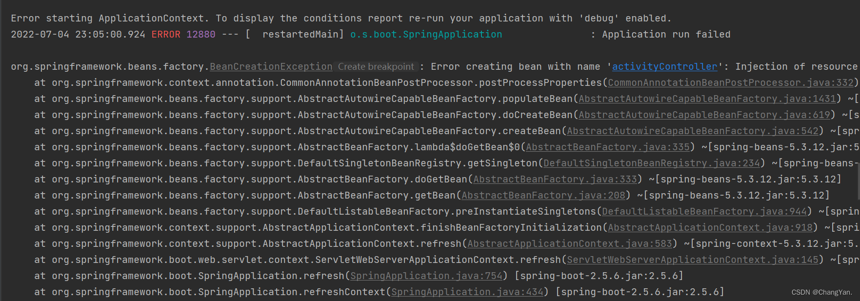
@TableId can‘t more than one in Class: “com.example.CloseContactSearcher.entity.Activity“.
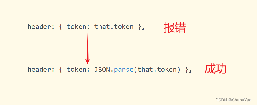
JWT signature does not match locally computed signature. JWT validity cannot be asserted and should
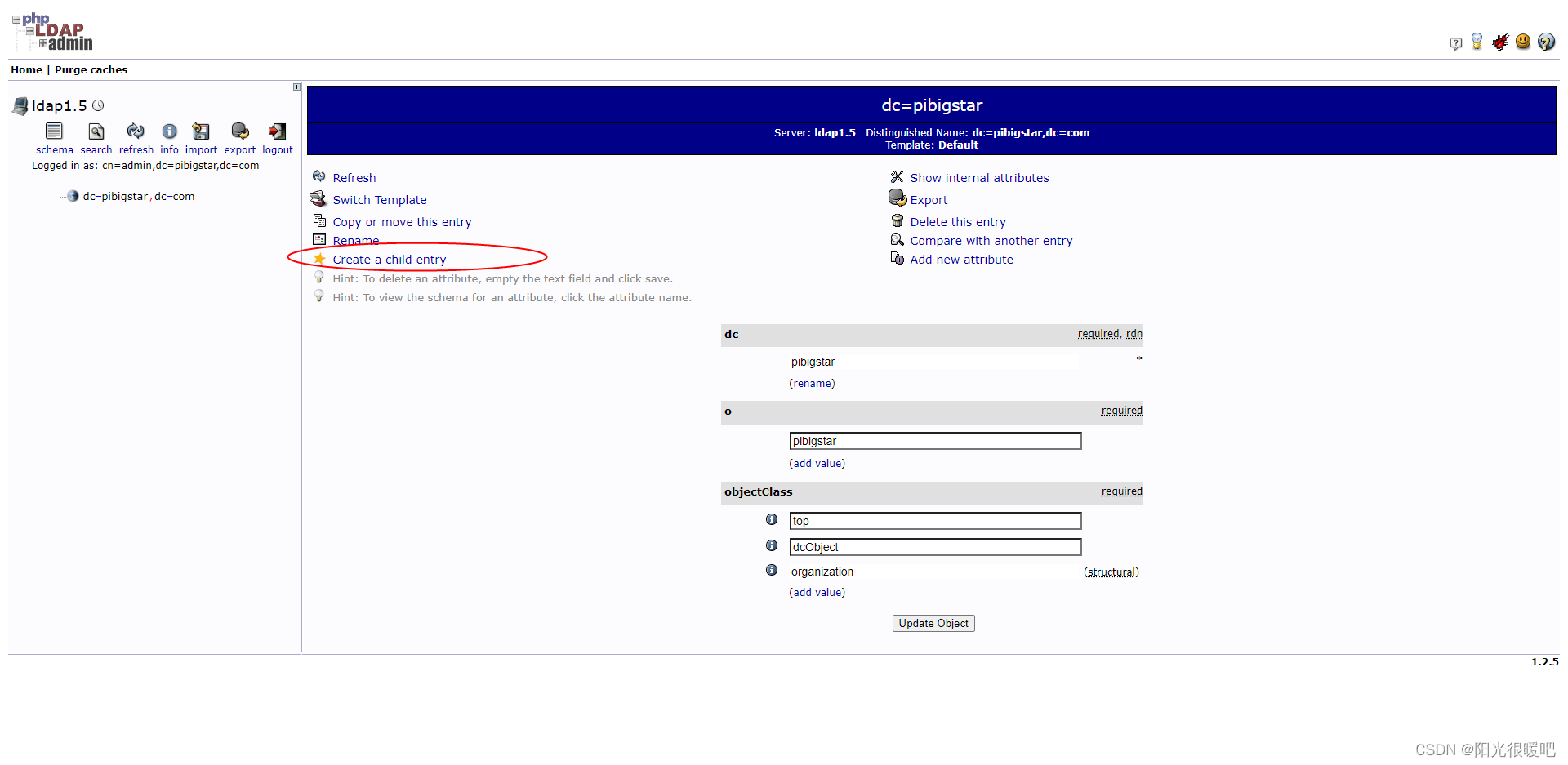
ldap创建公司组织、人员
随机推荐
Three sentences to briefly introduce subnet mask
DAY TWO
Personal digestion of DDD
Business process testing based on functional testing
uniapp中redirectTo和navigateTo的区别
工程师如何对待开源 --- 一个老工程师的肺腑之言
SQL的一种写法,匹配就更新,否则就是插入
openresty ngx_lua子请求
System activity monitor ISTAT menus 6.61 (1185) Chinese repair
Win10 startup error, press F9 to enter how to repair?
【CVPR 2022】半监督目标检测:Dense Learning based Semi-Supervised Object Detection
Racher integrates LDAP to realize unified account login
Interface master v3.9, API low code development tool, build your interface service platform immediately
Rails 4 asset pipeline vendor asset images are not precompiled
2022/2/12 summary
【vulnhub】presidential1
How to set encoding in idea
How engineers treat open source -- the heartfelt words of an old engineer
509 certificat basé sur Go
Core knowledge of distributed cache