[wave modeling 1] theoretical analysis and MATLAB simulation of wave modeling

1. Software version

matlab2017b

2. System principle

        The design of ocean wave modeling mainly involves the determination of ocean wave model , Calculation of various parameters of ocean waves , This system ,

The wave model is as follows ：

        In reality , There are many kinds of wave models , This model is used here , Mainly because the effect of this model is the closest to the effect on the website you give .

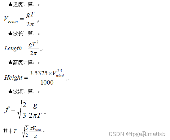
 G Is the acceleration of gravity , Take the constant 9.8

3. Core source code

global Winds;   % The wind speed 
global g; % Acceleration of gravity 
global kk; % The size ratio between the sand table of the simulation model and the actual area 
global Xmax;
global Ymax;
global Dxy;
global flag;
global VX;
global VY;
global VZ;


flag = 0;

g    = 9.8; % Acceleration of gravity 
kk   = 1/40; % The size ratio between the sand table of the simulation model and the actual area 
% Interval of simulation 
Dxy  = 4;


% The sea area covered by the simulation 
Xmax = 1000;
Ymax = 1000;

Start  = 200;
x      = [Start:Dxy:Xmax];
Ymax2  = round(Ymax/2);
y      = [Start:Dxy:Ymax2];
[xo,yo]= meshgrid(x,y);
z2     = zeros(size(x));

% The wave height of the wave itself 
r = (3.5325*Winds^2.5)/1000;

% The wave length of the wave itself 
k = 2*g/(3*Winds^2);
L = 2*pi/k;

% cycle T
T = sqrt(2*pi*L/g);

% Wave frequency 
w = sqrt(2/3)*g/T;
t = 0;

while(flag == 0)
    disp('the wind speed is');Winds
    t = t + 1;
    for i = 1:(Ymax2-Start)/Dxy+1
        for j = 1:(Xmax-Start)/Dxy+1
            % Attenuation coefficient 
            d             = sqrt((xo(1,j)-0)^2 + (yo(1,j)-0)^2);
            alphas        = exp(-0.07*d) - 0.18; 
            z2(i,j)       = alphas*r*cos(k*sqrt((xo(1,j)-0)^2 + (yo(1,j)-0)^2) - w*t);
        end
    end
    % Show local effects 
    axes(handles.axes1);
    surfl(xo,yo,z2);
    axis([Start-50 Xmax+50 Start-50 Ymax2+50 -8 10]);
    shading interp;
    colormap([143/255,157/255,203/255]);
    alpha(0.75);
    lightangle(-30,90);
    
    view([VX,VY,VZ]);
    
    
    pause(0.1);    
    
    
    % The wave length of the wave itself 
    k = 2*g/(3*Winds^2);
    Ls = 2*pi/k;
    set(handles.edit1,'String',num2str(Ls));
    
    
    % Calculate the parameter index of the wave 
    % The wave height of the wave itself 
    rs = (3.5325*Winds^2.5)/1000;
    set(handles.edit3,'String',num2str(rs));
    

    % cycle T
    T = sqrt(2*pi*L/g);
    % Speed 
    c = g*T/(2*pi); 
    set(handles.edit4,'String',num2str(c)); 
    
    % Wave frequency 
    w = sqrt(2/3)*g/T;    
    set(handles.edit5,'String',num2str(w/2/pi));
    
end

4. test result

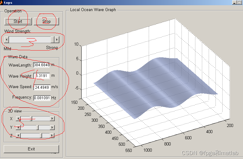
The simulation operation is shown in the above figure ,

First click on START Start simulating the effect of waves , And then click stop Can pause .

Upper figure 3 The tag is the corresponding button on the website to adjust the wind speed .

4 All parameters of the wave are displayed . See the theoretical introduction on the previous page for the calculation of specific parameters

5 Here is 3D Display of effect , You can observe the waves from different angles （MATLAB in GUI Of AXIS It is impossible to rotate the mouse directly for 3D display , So you need to display through this function ）

A19-06