Sequence model

• In the time series model , Current data is related to previously observed data
• Autoregressive models use their own past data to predict the future
• The Markov model assumes that it is currently only related to a few recent data , And then simplify the model
• Latent variable model uses latent variables to summarize historical information

Import related packages

import torch
from torch import nn
from d2l import torch as d2l
import matplotlib.pyplot as plt

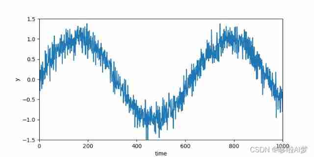
Use sine function and some additive noise to generate sequence data

T = 1000  # Total points 
x = torch.arange(1,T+1,dtype=torch.float32)
y = torch.sin(0.01*x)+torch.normal(0,0.2,(T,))
plt.figure(figsize=(8,4))
plt.xlim((0,1000))
plt.ylim((-1.5,1.5))
plt.xlabel('time')
plt.ylabel('y')
plt.plot(x,y)
plt.show()

The model predicts the next time step

#PyTorch Data Iterative loading 
def load_array(data_arrays,batch_size,is_train=True):
    dataset = TensorDataset(*data_arrays)
    return DataLoader(dataset,batch_size,shuffle=is_train)
# The sequence is transformed into a model “ features - label ”
tau = 4
features = torch.zeros((T - tau, tau))
for i in range(tau):
    features[:, i] = x[i:T - tau + i]
labels = x[tau:].reshape((-1, 1))

batch_size, n_train = 16, 600
train_iter = d2l.load_array((features[:n_train], labels[:n_train]),
                            batch_size, is_train=True)

# Initialize the function of network weight 
def init_weights(m):
    if type(m) == nn.Linear:
        nn.init.xavier_uniform_(m.weight)

#MPL
def get_net():
    net = nn.Sequential(
        nn.Linear(4,10),
        nn.ReLU(),
        nn.Linear(10,1)
    )
    net.apply(init_weights)
    return net

def evaluate_loss(net, data_iter, loss):
    metric = d2l.Accumulator(2) #  The sum of the losses , Number of samples 
    for X, y in data_iter:
        out = net(X)
        y = y.reshape(out.shape)
        l = loss(out, y)
        metric.add(l.sum(), l.numel())
    return metric[0] / metric[1]

# Training 
def train(net,train_iter,loss,epochs,lr):
    optimilizer = torch.optim.Adam(net.parameters(),lr)
    for epoch in range(epochs):
        for X,y in train_iter:
            optimilizer.zero_grad()
            l = loss(net(X),y)
            l.sum().backward()
            optimilizer.step()
        print(f'epoch {
      epoch + 1}, '
              f'loss: {
      evaluate_loss(net, train_iter, loss):f}')

loss = nn.MSELoss(reduction='none')
net = get_net()
train(net,train_iter,loss,10,0.01)

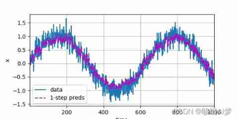
onestep_preds = net(features)
d2l.plot(
    [time, time[tau:]],
    [x.detach().numpy(), onestep_preds.detach().numpy()], 'time', 'x',
    legend=['data', '1-step preds'], xlim=[1, 1000], figsize=(6, 3))
d2l.plt.show()

Multi step prediction

max_steps = 64

features = torch.zeros((T - tau - max_steps + 1, tau + max_steps))
for i in range(tau):
    features[:, i] = x[i:i + T - tau - max_steps + 1]

for i in range(tau, tau + max_steps):
    features[:, i] = net(features[:, i - tau:i]).reshape(-1)

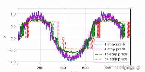
steps = (1, 4, 16, 64)
d2l.plot([time[tau + i - 1:T - max_steps + i] for i in steps],
         [features[:, (tau + i - 1)].detach().numpy() for i in steps], 'time',
         'x', legend=[f'{
      i}-step preds'
                      for i in steps], xlim=[5, 1000], figsize=(6, 3))

summary ：

• For a causal model where time is advancing , Positive estimation usually ⽐ Reverse estimation is easier .
• For up to time steps t The sequence of observations , It is in the time step t + k The predicted output is “k Next step prediction ”. As we predict the time k An increase in value , It will cause the rapid accumulation of errors and the rapid decline of prediction quality .