当前位置:网站首页>移动机器人路径规划:人工势场法[通俗易懂]
移动机器人路径规划:人工势场法[通俗易懂]
2022-07-02 18:10:00 【全栈程序员站长】
大家好,又见面了,我是你们的朋友全栈君。
人工势场法是一种原理比较简单的移动机器人路径规划算法,它将目标点位置视做势能最低点,将地图中的障碍物视为势能高点,计算整个已知地图的势场图,然后理想情况下,机器人就像一个滚落的小球,自动避开各个障碍物滚向目标点。
具体地,目标点的势能公式为:
其中写道,为防止距离目标点较远时的速度过快,可以采用分段函数的形式描述,后文会进行展示。 而障碍物的势能表示为:
即在障碍物周围某个范围内具有高势能,范围外视障碍物的影响为0。 最终将目标点和障碍物的势能相加,获得整张势能地图:
以下是参考链接中的源代码,比较容易懂:
""" Potential Field based path planner author: Atsushi Sakai (@Atsushi_twi) Ref: https://www.cs.cmu.edu/~motionplanning/lecture/Chap4-Potential-Field_howie.pdf """

from collections import deque
import numpy as np
import matplotlib.pyplot as plt

# Parameters
KP = 5.0  # attractive potential gain
ETA = 100.0  # repulsive potential gain
AREA_WIDTH = 30.0  # potential area width [m]
# the number of previous positions used to check oscillations
OSCILLATIONS_DETECTION_LENGTH = 3

show_animation = True


def calc_potential_field(gx, gy, ox, oy, reso, rr, sx, sy):
    """ 计算势场图 gx,gy: 目标坐标 ox,oy: 障碍物坐标列表 reso: 势场图分辨率 rr: 机器人半径 sx,sy: 起点坐标 """
    # 确定势场图坐标范围:
    minx = min(min(ox), sx, gx) - AREA_WIDTH / 2.0
    miny = min(min(oy), sy, gy) - AREA_WIDTH / 2.0
    maxx = max(max(ox), sx, gx) + AREA_WIDTH / 2.0
    maxy = max(max(oy), sy, gy) + AREA_WIDTH / 2.0
    # 根据范围和分辨率确定格数:
    xw = int(round((maxx - minx) / reso))
    yw = int(round((maxy - miny) / reso))

    # calc each potential
    pmap = [[0.0 for i in range(yw)] for i in range(xw)]

    for ix in range(xw):
        x = ix * reso + minx   # 根据索引和分辨率确定x坐标

        for iy in range(yw):
            y = iy * reso + miny  # 根据索引和分辨率确定x坐标
            ug = calc_attractive_potential(x, y, gx, gy)  # 计算引力
            uo = calc_repulsive_potential(x, y, ox, oy, rr)  # 计算斥力
            uf = ug + uo
            pmap[ix][iy] = uf

    return pmap, minx, miny


def calc_attractive_potential(x, y, gx, gy):
    """ 计算引力势能:1/2*KP*d """
    return 0.5 * KP * np.hypot(x - gx, y - gy)


def calc_repulsive_potential(x, y, ox, oy, rr):
    """ 计算斥力势能: 如果与最近障碍物的距离dq在机器人膨胀半径rr之内:1/2*ETA*(1/dq-1/rr)**2 否则:0.0 """
    # search nearest obstacle
    minid = -1
    dmin = float("inf")
    for i, _ in enumerate(ox):
        d = np.hypot(x - ox[i], y - oy[i])
        if dmin >= d:
            dmin = d
            minid = i

    # calc repulsive potential
    dq = np.hypot(x - ox[minid], y - oy[minid])

    if dq <= rr:
        if dq <= 0.1:
            dq = 0.1

        return 0.5 * ETA * (1.0 / dq - 1.0 / rr) ** 2
    else:
        return 0.0


def get_motion_model():
    # dx, dy
    # 九宫格中 8个可能的运动方向
    motion = [[1, 0],
              [0, 1],
              [-1, 0],
              [0, -1],
              [-1, -1],
              [-1, 1],
              [1, -1],
              [1, 1]]

    return motion


def oscillations_detection(previous_ids, ix, iy):
    """ 振荡检测:避免“反复横跳” """
    previous_ids.append((ix, iy))

    if (len(previous_ids) > OSCILLATIONS_DETECTION_LENGTH):
        previous_ids.popleft()

    # check if contains any duplicates by copying into a set
    previous_ids_set = set()
    for index in previous_ids:
        if index in previous_ids_set:
            return True
        else:
            previous_ids_set.add(index)
    return False


def potential_field_planning(sx, sy, gx, gy, ox, oy, reso, rr):

    # calc potential field
    pmap, minx, miny = calc_potential_field(gx, gy, ox, oy, reso, rr, sx, sy)

    # search path
    d = np.hypot(sx - gx, sy - gy)
    ix = round((sx - minx) / reso)
    iy = round((sy - miny) / reso)
    gix = round((gx - minx) / reso)
    giy = round((gy - miny) / reso)

    if show_animation:
        draw_heatmap(pmap)
        # for stopping simulation with the esc key.
        plt.gcf().canvas.mpl_connect('key_release_event',
                lambda event: [exit(0) if event.key == 'escape' else None])
        plt.plot(ix, iy, "*k")
        plt.plot(gix, giy, "*m")

    rx, ry = [sx], [sy]
    motion = get_motion_model()
    previous_ids = deque()

    while d >= reso:
        minp = float("inf")
        minix, miniy = -1, -1
        # 寻找8个运动方向中势场最小的方向
        for i, _ in enumerate(motion):
            inx = int(ix + motion[i][0])
            iny = int(iy + motion[i][1])
            if inx >= len(pmap) or iny >= len(pmap[0]) or inx < 0 or iny < 0:
                p = float("inf")  # outside area
                print("outside potential!")
            else:
                p = pmap[inx][iny]
            if minp > p:
                minp = p
                minix = inx
                miniy = iny
        ix = minix
        iy = miniy
        xp = ix * reso + minx
        yp = iy * reso + miny
        d = np.hypot(gx - xp, gy - yp)
        rx.append(xp)
        ry.append(yp)
        # 振荡检测,以避免陷入局部最小值:
        if (oscillations_detection(previous_ids, ix, iy)):
            print("Oscillation detected at ({},{})!".format(ix, iy))
            break

        if show_animation:
            plt.plot(ix, iy, ".r")
            plt.pause(0.01)

    print("Goal!!")

    return rx, ry


def draw_heatmap(data):
    data = np.array(data).T
    plt.pcolor(data, vmax=100.0, cmap=plt.cm.Blues)


def main():
    print("potential_field_planning start")

    sx = 0.0  # start x position [m]
    sy = 10.0  # start y positon [m]
    gx = 30.0  # goal x position [m]
    gy = 30.0  # goal y position [m]
    grid_size = 0.5  # potential grid size [m]
    robot_radius = 5.0  # robot radius [m]
    # 以下障碍物坐标是我进行修改后的,用来展示人工势场法的困于局部最优的情况:
    ox = [15.0, 5.0, 20.0, 25.0, 12.0, 15.0, 19.0, 28.0, 27.0, 23.0, 30.0, 32.0]  # obstacle x position list [m]
    oy = [25.0, 15.0, 26.0, 25.0, 12.0, 20.0, 29.0, 28.0, 26.0, 25.0, 28.0, 27.0]  # obstacle y position list [m]

    if show_animation:
        plt.grid(True)
        plt.axis("equal")

    # path generation
    _, _ = potential_field_planning(
        sx, sy, gx, gy, ox, oy, grid_size, robot_radius)

    if show_animation:
        plt.show()


if __name__ == '__main__':
    print(__file__ + " start!!")
    main()
print(__file__ + " Done!!")人工势场法的一项主要缺点就是可能会落入局部最优解,下图是源代码运行后的结果:
下面是在我添加了一些障碍物后,人工势场法困于局部最优解的情况:虽然还没有到达目标点,但势场决定了路径无法再前进。
需要注意的是,源代码在计算目标点势场的时候,使用的是某x,y位置距离目标点的距离的一次项,并未如课件中所示使用二次项,也是为了使势场变化没有那么快。下面是按照课件中所说,使用距离的二次项运行的结果,我们可以看到,为运行正常,KP需要调得很低:
KP = 0.1
def calc_attractive_potential(x, y, gx, gy):
    """ 计算引力势能:1/2*KP*d^2 """
return 0.5 * KP * np.hypot(x - gx, y - gy)**2正常运行:
困在局部最优点:
可以从势场图中看到,引力变化较上一个例子快得多。
最后,我们将程序修改成上面课件截图中所示的分段函数:
KP = 0.25
dgoal = 10
def calc_attractive_potential(x, y, gx, gy):
    """ 计算引力:如课件截图 """
    dg = np.hypot(x - gx, y - gy)
    if dg<=dgoal:
        U = 0.5 * KP * np.hypot(x - gx, y - gy)**2
    else:
        U = dgoal*KP*np.hypot(x - gx, y - gy) - 0.5*KP*dgoal
return U正常运行:
困于局部最优:
可以看到引力势场分段的效果。
发布者:全栈程序员栈长,转载请注明出处:https://javaforall.cn/148611.html原文链接:https://javaforall.cn
边栏推荐
- Golang concurrent programming goroutine, channel, sync
- Excel如何进行隔行复制粘贴
- PyTorch函数中的__call__和forward函数
- 迷你高尔夫球场:伦敦休闲旅游好去处
- Stm32g0 USB DFU upgrade verification error -2
- 预处理和预处理宏
- How to delete the border of links in IE? [repeat] - how to remove borders around links in IE? [duplicate]
- 中国信通院《数据安全产品与服务图谱》,美创科技实现四大板块全覆盖
- Transformation of thinking consciousness is the key to the success or failure of digital transformation of construction enterprises
- 教程篇(5.0) 09. RESTful API * FortiEDR * Fortinet 网络安全专家 NSE 5
猜你喜欢

潇洒郎:彻底解决Markdown图片问题——无需上传图片——无需网络——转发给他人图片无缺失
Introduction to the paper | analysis and criticism of using the pre training language model as a knowledge base
【JVM调优实战100例】03——JVM堆调优四例
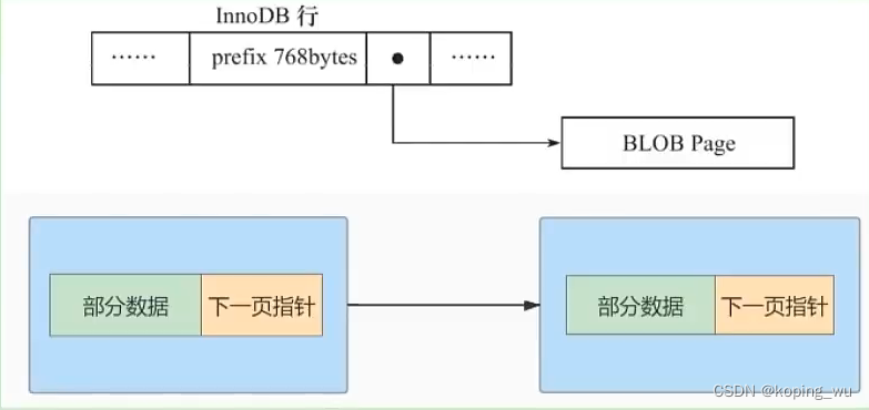
MySQL advanced learning summary 8: overview of InnoDB data storage structure page, internal structure of page, row format
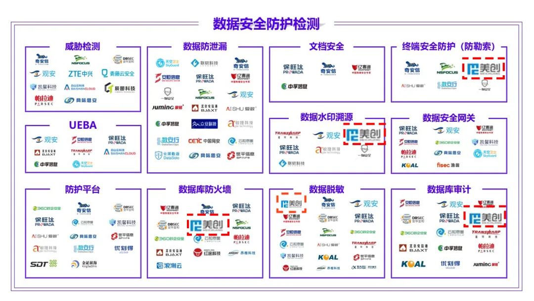
According to the atlas of data security products and services issued by the China Academy of information technology, meichuang technology has achieved full coverage of four major sectors
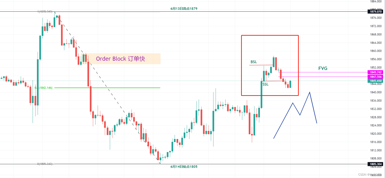
Exness in-depth good article: dynamic series - Case Analysis of gold liquidity (V)
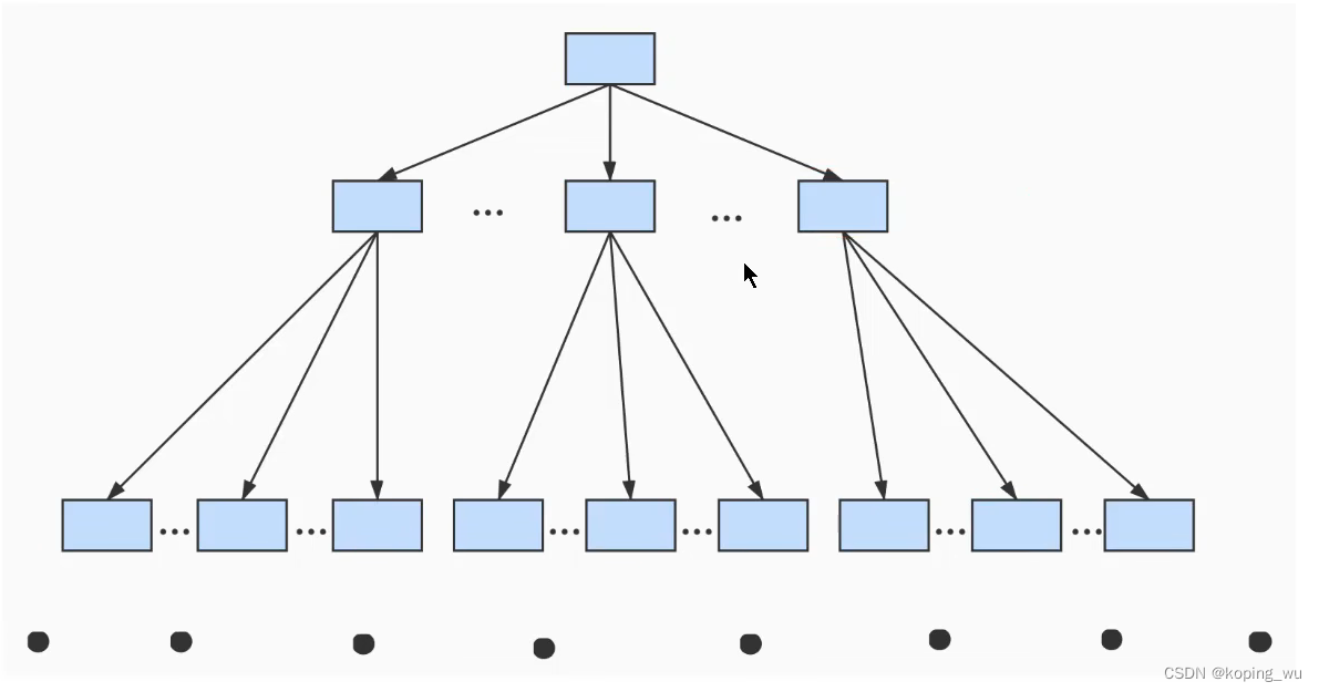
Mysql高级篇学习总结6:索引的概念及理解、B+树产生过程详解、MyISAM与InnoDB的对比
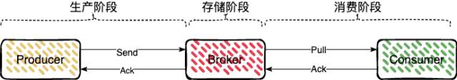
消息队列消息丢失和消息重复发送的处理策略
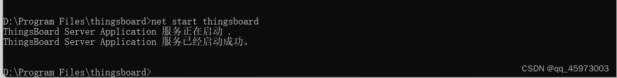
Installation of thingsboard, an open source IOT platform

STM32G0 USB DFU 升级校验出错-2
随机推荐
ICDE 2023|TKDE Poster Session(CFP)
【JVM调优实战100例】02——虚拟机栈与本地方法栈调优五例
[test development] takes you to know what software testing is
为什么要做企业固定资产管理系统,企业如何加强固定资产管理
预处理和预处理宏
Compile oglpg-9th-edition source code with clion
【JVM调优实战100例】03——JVM堆调优四例
电商系统中常见的 9 大坑,你踩过没?
PyTorch函数中的__call__和forward函数
Markdown basic grammar
Transformation of thinking consciousness is the key to the success or failure of digital transformation of construction enterprises
使用CLion编译OGLPG-9th-Edition源码
Tutorial (5.0) 09 Restful API * fortiedr * Fortinet network security expert NSE 5
拦截器与过滤器的区别
MySQL高级(进阶)SQL语句
仿京东放大镜效果(pink老师版)
R language uses the lsnofunction function function of epidisplay package to list all objects in the current space, except user-defined function objects
Excel如何进行隔行复制粘贴
Progress-进度条
2022.7.1-----leetcode.241