Scoring prediction problem

So far we have been discussing TopN recommend , That is, given a user , How to generate a length of N A list of recommendations , Make the recommendation list meet the interests and needs of users as much as possible . however , Many students engaged in recommendation system research first came into contact with the problem of score prediction . Score prediction is the core of recommendation system research . The most basic data set of scoring prediction problem is the user scoring data set . This data set consists of user scoring records , Each score record is a triple （u,i,r）, Represent user u Give the item i Given a score r. Because it is impossible for users to rate all items , Therefore, the scoring prediction problem is how to predict unknown user scoring records through known user historical scoring records .

Off line experimental method

Scoring prediction problems are basically studied through off-line experiments . Researchers will build a user interest model based on the test set to predict the user scores in the test set . For a pair of users and items in the test set （U,i）, user U For items i Your true score is r, And users who recommend algorithm prediction U For items i The score of is r’, Then we can generally use the root mean square error RMSE Measure the accuracy of the forecast ：

The goal of score prediction is to find the best model to minimize the test set RMSE.

Scoring prediction algorithm

Average

The simplest scoring prediction algorithm is to use the average value to predict the user's rating of items . The different averages are described below .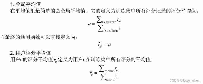


Global average , Both the average user score and the average item score are special cases of the class average .

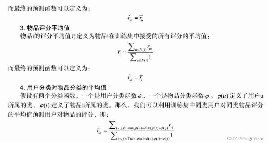
In addition to this 3 A special average , Many different classification functions can be defined on the user rating data .
Average score of users and items ： For a user , You can calculate his average score . Then sort all users according to their average scores from small to large , And divide the users into items according to the average score, which can also be classified in the same way .
User activity and item popularity ： For a user , Define the number of items he scores as his activity . After getting the user activity , Users can be sorted from small to large by activity , Then the average score is N class . The popularity of an item is defined as the number of users who rate the item , Items can also be divided evenly according to popularity N class .

Domain based approach

arwar utilize MovieLens The smallest data set pair 3 The similarity of the two methods is compared , And will MAE As a measure . The experimental results show that the modified cosine similarity can be used to predict the best score MAE. But here's the thing , Experiments on one dataset do not mean that the same results can be obtained on other datasets .

Implicit semantic model and matrix decomposition

In the field of recommendation systems , The most frequently mentioned are the latent semantic model and the matrix decomposition model . Actually , These two nouns mean the same thing , It is how to complete the score matrix by reducing dimension . The user's rating behavior can be expressed as a rating matrix R, among R[u][i] Is the user u For items i The score . however , use Users will not rate all items , So many elements in this matrix are empty , These empty elements are called missing values (missing value). therefore , In a sense, scoring prediction means filling in the blanks , If a user doesn't over rate an item , Then the recommendation system should predict whether the user will rate the item and how much it will rate .

1. Conventional SVD decompose

How to complete a matrix , There have been many studies in history . There are many ways to complete an empty matrix , And we What we are looking for is a complement method that minimizes matrix perturbation . So what is the minimum disturbance to the matrix ？ It is generally believed , If The eigenvalues of the matrix after completion are almost the same as those of the matrix before completion , Even if the disturbance is small . therefore , The earliest matrix The decomposition model is mathematically SVD ( Singular value decomposition ) At the beginning . Given w Users and n Items , And the user's rating matrix for the items R. First, you need to simply complete the missing values in the scoring matrix , For example, use the global average , Get the completed matrix R’. next , It can be used SVD Decomposition will R’ Decompose into the following forms ：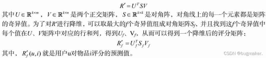

SVD Decomposition is a commonly used matrix decomposition method in early recommendation system research , However, this method has the following disadvantages , So it's hard to be in Application in actual system .

1. This method first needs a simple method to complete the sparse scoring matrix . Generally speaking , The scoring matrix in the recommendation system is very sparse , Generally there are 95% The above elements are missing . And once completed , The scoring matrix becomes a A dense matrix , Thus, the storage of scoring matrix needs a very large space , This kind of space demand is in the actual system It is impossible to accept .
2. This method relies on SVD The computational complexity of the decomposition method is very high , Especially on dense large-scale matrices, it's very slow . Generally speaking , there SVD Decomposition is used for 1000 Matrices with dimensions above are already very slow , But the actual system moves There are tens of millions of users and millions of items , So this method cannot be used .

2. Simon Funk Of SVD decompose

Because of the above two shortcomings ,SVD The decomposition algorithm has not been widely concerned in the field of recommendation system for several years . until Simon Funk An algorithm was posted on the blog Latent Factor Model ( Referred to as LFM )
From the perspective of matrix decomposition , If we put the scoring matrix R It is decomposed into two low dimensional matrices and multiplied ：


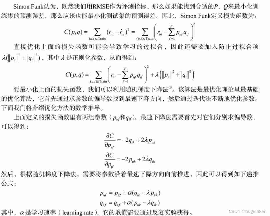
LearningLFM It mainly includes two steps . First , Need to be right p、q Initialize the matrix , Then we need to get the final result through the iteration of the random gradient descent method p,q matrix .
LFM It has been a great success since it was put forward , Later, many famous models were made by LFM What you get by tinkering , The following will introduce the improvements LFM Various methods of .

3. After adding the paranoid item LFM

This prediction formula has been added 3 term u、bu、bi. We call this model BiasSVD. The functions of the three newly added items in this model are as follows .

u： The global average of all recorded scores in the training set . In different websites , Because the location of the website is different from the items sold , The overall score distribution of the website will also show some differences . For example, users in some websites just like to play High marks , Users of other websites just like to give low scores . The global average can represent the website's own evaluation of users The influence of points .
bu： User bias (user bias) term . This item indicates that users' scoring habits have nothing to do with items factors . For example, some users are more demanding , It's very demanding of everything , Then his score will be lower ,
Some users are more tolerant , Feel good about everything , Then his score will be on the high side .
bi： Item offset (item bias) term . This item indicates that the item acceptance score has nothing to do with the user factors . For example, some items are of high quality , Therefore, the scores obtained are relatively high , And some objects themselves The quality is poor , Therefore, the scores obtained will be relatively low .

4. Considering the influence of neighborhood LFM

Ahead LFM The model does not explicitly consider the impact of users' historical behavior on users' score prediction . So ,Koren stay Netflix Prize In the competition, a model is proposed to add the items scored by the user's history to LFM In the model ,Koren Call this model SVD++.
Introducing SVD++ Before , First, let's discuss how to make the neighborhood based method look like LFM So design a model that you can learn . We can ItemCF The prediction algorithm is changed as follows ：

Add time information

Researchers have proposed a method to reduce prediction error by using time information . There are two ways to use time information , One is to apply the time information to the neighborhood based model , The other is to apply the time information to the matrix decomposition model . These two algorithms will be introduced respectively .

1. Neighborhood based models fuse temporal information
   because NetflixPrize The number of users in the dataset is too large , So user based neighborhood model is rarely used , This is mainly because it is very difficult to store the user similarity matrix . therefore , This section mainly discusses how to fuse time information into the item based neighborhood model .
   Netflix Prize Our team BigChaos A neighborhood based model incorporating time information is mentioned in the technical report , This section calls this model TItemCF. The algorithm predicts what the user will give to the item at a certain time by the following formula ：
   
2. The model based on matrix decomposition fuses time information
   After introducing the time information , The user rating matrix is no longer a two-dimensional matrix , It becomes a three-dimensional matrix . however , We can decompose the three-dimensional matrix in the same way as the two-dimensional matrix . Let's review the previous BiasSVD Model ：
   

Model fusion

Netflix Prize The final winning team achieved the final success by integrating the results of hundreds of models . It can be seen that model fusion is very important to improve the accuracy of scoring prediction . This section discusses two different techniques for model fusion .

As can be seen from the above description , Cascading fusion is much like Adaboost Algorithm . and Adaboost Similar algorithm , This method produces a new model each time , Add certain parameters to the old model , Thus, the training set error is minimized . The difference is , Here every The sample set is not sampled when a new model is generated , For those samples whose predictions are wrong , Instead, the full sample set is used every time forecast , But the model used each time is different .
Generally speaking , Cascade fusion methods are used for simple predictors , For example, the average predictor mentioned earlier .

Generally speaking , The solution of scoring prediction problem needs training on training set K Different predictors , Then make predictions on the test set . however , If we continue to merge on the training set K A predictor , Get the linear weighting coefficient , It will cause the problem of over fitting . therefore , The following methods are generally used in model fusion .

1. Assume that the data set has been divided into training sets A And test set B So first you need to put the training set A According to the same segmentation method, it is divided into A1 and A2, among A2 Generation method and B The generation method of is consistent , And similar in size .
2. stay A1 Training K Different predictors , stay A2 Make predictions on . Because we know A2 The true score on the , So it can be A2 The linear fusion coefficient is calculated by the least square method α.
3. stay A Training K Different predictors , stay B Make predictions on , And put this K A predictor is B The prediction results on the are weighted and fused according to the obtained linear fusion coefficients , To get the final prediction results .
   Except for linear fusion , There are many complex fusion methods , For example, using the fusion algorithm of artificial neural network . Actually , Model Fusion problem is a typical regression problem , Therefore, all regression algorithms can be used for model fusion .