Introduction Guide to stereo vision (6): level constraints and polar correction of fusiello method

Dear students , Our world is 3D The world , Our eyes can observe three-dimensional information , Help us perceive distance , Navigation obstacle avoidance , So as to soar between heaven and earth . Today's world is an intelligent world , Our scientists explore a variety of machine intelligence technologies , Let the machine have the three-dimensional perception of human beings , And hope to surpass human beings in speed and accuracy , For example, positioning navigation in autopilot navigation , Automatic obstacle avoidance of UAV , Three dimensional scanning in the measuring instrument, etc , High intelligent machine intelligence technology is 3D Visual realization .

Stereo vision is an important direction in the field of 3D reconstruction , It simulates the structure of the human eye and simulates the binocular with two cameras , Project in Perspective 、 Based on triangulation , Through the logical complex homonymous point search algorithm , Restore the 3D information in the scene . It is widely used , Autopilot 、 Navigation obstacle avoidance 、 Cultural relic reconstruction 、 Face recognition and many other high-tech applications have its key figure .

This course will help you to understand the theoretical and practical knowledge of stereo vision from simple to profound . We will talk about the coordinate system and camera calibration , From passive stereoscopic to active stereoscopic , Even from deep recovery to grid construction and processing , Interested students , Come and explore the charm of stereovision with me ！

This course is an electronic resource , So there will not be too many restrictions in the writing , But it will be logically clear 、 Easy to understand as the goal , Level co., LTD. , If there are deficiencies , Please give me some advice ！
Personal wechat ：EthanYs6, Add me to the technical exchange group StereoV3D, Talk about technology together .
CSDN Search for ：Ethan Li Li Yingsong , see Web based courses .
Lesson code , Upload to github On , Address ：StereoV3DCode：https://github.com/ethan-li-coding/StereoV3DCode

I've kept you waiting , Recent job changes , Still adapting , I hope you have a lot of ！

In the previous post , We have covered the basics and camera calibration , Students must be thinking about which direction to go next , After camera calibration , The pose of the camera is determined , And then , It's natural to take pictures with a camera , After collecting the images ？ What should we do ？

Back to the ultimate goal of stereovision , It calculates the three-dimensional coordinates of the scene by double view matching of the image , In this introductory series , I have to explain in advance what is Binocular matching , Especially the meaning of "match" .

matching , English is match, Literally , Yes, it will N（N>=2） Two goals go together , this N Goals usually have some common or similar attributes , For example, the left and right of a pair of headphones , They belong to the same pair of earphones , Like you and your brothers and sisters , You are all your parents' children . Naturally , Binocular matching , In two views , Find pixel pairs with common attributes , In stereovision , This common attribute is ： They are projections of the same point in space in their respective views , That is, they represent the same point in space .

Then why do you want to do double view matching ？ It starts with triangulation ,

Triangulation is a very simple concept , It refers to the determination of two points and the rays starting from two points , You can calculate the coordinates of another point where the two rays intersect , Three points form a triangle , So it is called triangulation .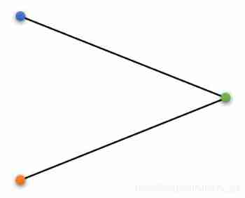

Corresponding to stereo vision , The three points are ： The optical center point of two cameras and a spatial point , The position of the optical center is determined by calibration , The two rays are the connecting lines between the two optical centers and the space points , If two more rays are identified , You can calculate the coordinates of the space points , Someone asked , How to determine two rays ？ That's what the match has to do .

Let's add something to the picture above , The two points on the left are the optical centers of the two cameras $C$, A point on the right is a spatial point $P$, Add an image plane in front of the optical center $I$（ As I said in my previous blog post , What looks like a plane is actually behind the optical center , To get to the front is equivalent , But it's more intuitive to understand ）. The intersection of the line between the space point and the optical center and the image plane is $p$.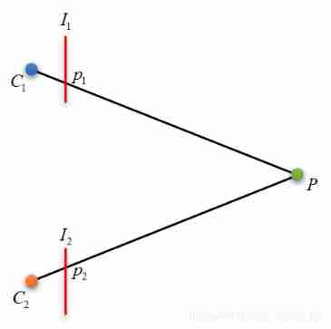

On the other hand ,$p$ It's a space point $P$ Projection point on the image , That is, we see the image of the object on the image .

Okay , Back to the previous question , How to determine the ray $C_{1}P,C_{2}P$ Well ？ obviously , An obvious identity relationship in the figure is ,$C_{1}P\equiv C_1{p}_1,C_{2}P\equiv C_2{p}_2$, So determine the ray $C_{1}P,C_{2}P$ It can be converted into definite rays $C_1{p}_1,C_2{p}_1$.$C_1,C_2$ We have got through calibration , and $p_1,p_2$ The process of determining is called matching . In general , We give a pixel $p_1$, Find the corresponding matching point in another view $p_2$, Once you find it, you can calculate $P$ 了 .

Okay , That's all for the definition of matching . Let's go back to today's theme ： A contrapolar constraint .

Why study contrapolar constraints

In computer science , Given a definite problem , There must be various algorithms to study how to solve it , Then it comes to how to solve it efficiently , And they don't go in sequence , But cross , That is, the study of the most definite solution and the study of the most efficient solution are carried out simultaneously . For the matching problem , Find the corresponding matching point for this problem , It's not a simple problem , For decades, , No one algorithm can find all the right matching pairs perfectly , The angle produces affine distortion between images 、 Weak texture 、 Repeat texture 、 Dark light 、 Overexposure 、 Transparency, etc , There are a lot of headaches , And some seem to have no solution , However, this does not prevent many scholars from studying this issue , So many excellent algorithms are produced , Many have been proved to be accurate and efficient in practical engineering applications （ The accuracy here does not mean that they are geometrically accurate , It means engineering precision ）.

Back to the point , Anyone familiar with the idea of optimization knows , When it comes to the word search space , Someone will naturally think of how to reduce the search space to improve the search efficiency , After all, our computer is designed by people in three-dimensional space , Its motion must also follow the law of three-dimensional space , No high-dimensional space folding ability , The search is still limited by the size and distance of the space , But there are a few things we can do ：

1. Make its motion space smaller .
2. Make it stay less where there is no target point .

our Level constraints Just to do the first thing , Make the matching search space smaller , Omit pixels that are completely impossible to solve . Simply speaking , Two pixels as a match , It must satisfy a constraint formula , If not, it is definitely not a matching point . This can save a lot of meaningless search , But a little regret , This constraint is not the only constraint , That is, for a pixel on the left view , There are still many pixels in the right view that meet this constraint , So we can only narrow the search space , The solution cannot be determined directly .

A contrapolar constraint , Is to constrain the search space to a straight line in the image plane , Let's talk about this slowly .

Polar plane and polar line

How did the antipolar constraint come about ？ Let's look at the picture below ：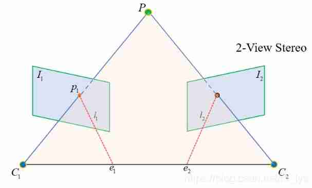

chart 1 Level constraints

Light heart $O_1,O_2$（ Forgive me for changing the symbol ） And spatial points $P$ Form a triangular relationship , In fact, they define a spatial plane , This plane intersects with both image planes , The intersection lines are $l_1,l_2$, Use our imagination , It's easy to see , stay $l_1$ All the points on the , His matching point must be $l_2$ On , This is the antipolar constraint , It limits the matching search space to a straight line , Greatly reduce the search space , Improve matching efficiency . And two straight lines $l_1,l_2$ It's called epipolar , We can call them both Polar pair . Remember this concept , There will be .

How to determine this straight line ？ We know $O_1,O_2,p$, You can calculate the plane $O_{1}p{O}_2$ The equation of , It's like a plane $I_2$（ Namely $p_2$ The image plane ） The intersecting straight line is $l_2$, With $l_2$ The equation of can be in the image plane $I_2$ Traverse the line one by one $l_2$ Pixels on . In sparse point matching , We can do this to improve search efficiency .

Epipolar correction

Okay , Above, we talked about level constraints , We understand its concept and spatial significance , Now I want to talk about an important concept ： Epipolar correction , The same question , Why talk about it , In the previous chapter we mentioned , Level constraints allow us to reduce the search space , With pair level constraints , For a pixel in the left view $p_1$, The matching points in the right view can be calculated $p_2$ The polar line where it is $l_2$, Thus in $l_2$ Search for the correct solution . Sounds really good , Greatly reduce the search space , But it still has one drawback , For each pixel to be matched in the left view , We have to calculate the corresponding polar line , If I have a lot of pixels to match （ This is the research direction of dense matching ： Match pixel by pixel ）, That's a lot of calculation .

Is there a way , You don't have to calculate , Directly determine the polar line on the right ？

The answer, of course, is , Epipolar correction Is to answer this question ！

Or look at the picture above , We will find further , Polar line $l_1$ All pixels and $l_2$ The pixels on satisfy the same constraint formula , That is to say, the polar line $l_1$ All pixels on , Calculated corresponding polar line , It's all the same $l_2$. The reason is , Because they all belong to the same polar plane ！ So you can think of it this way , One polar plane can find a pair of polar lines in two views , All pixels on this pair of epipolar lines satisfy the same constraint formula , Multiple polar planes generate multiple polar pairs , Many polar pairs can cover all pixels on the image ！

further , We can rearrange the pixels on these polar pairs in the image plane , Pixels on the same polar pair are arranged in the same row , In this way, we can determine the pixels of the same polar pair by line number , No need to calculate the polar equation . in short , Left view pixels $p_1$ The matching point of must be located in the row of pixels with the same row number in the right view .

The above is a simple explanation of epipolar correction . And geometrically , We have a more professional explanation ：

Epipolar correction is done by rotating two cameras , And redefine the new image plane , Let the epipolar pairs be collinear and parallel to a coordinate axis of the image plane （ Usually the horizontal axis ）, This operation also creates a new stereo pair . After correction , Same matching point pair , In the same row of both views , This means that they only have horizontal coordinates （ Or column coordinates ） The difference of , This difference is called parallax （ Abbreviation $d$）, Mathematically , parallax $d=col(p_1)-col(p_2)$（$col$ Refers to horizontal coordinates , Or column coordinates $）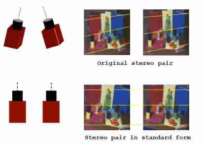

chart 2 Epipolar correction * picture source ：Mattoccia S , Updates S M , Outline S M . Stereo Vision: Algorithms and Applications[J]. 2011.*

This operation makes dense matching much easier , Of course , It's just relatively easy .

Explain the concept and significance of epipolar correction , Another thing we care about is , How to do epipolar correction ？

There are different ways to do this , Today we mainly talk about Fusiello Correction method .

Let's look at our goals first ：

1. A polar pair is parallel to a coordinate axis .
2. Polar pairs are collinear , The matching point pairs are located on the same row of the image plane .

To achieve these two goals , We need to do different analyses , It was said that , Epipolar correction is done by rotating the camera and redefining the image plane , actually , The essence of the two operations is to redefine the projection matrix $M=K[R|-RC]$. Redefine the rotation matrix by rotating the camera $R\to R_n$ Make the new image plane coplanar and parallel to the camera baseline , Can meet the goal 1, And redefine the internal parameters of the image plane $K\to K_n$ Make both cameras have the same internal parameters , Can meet the goal 2.

As shown in the figure below , Corrected image plane , level $u$ Axis and baseline $C_1{C}_2$ parallel , The focal length $f$ Equal to the coordinates of the principal point .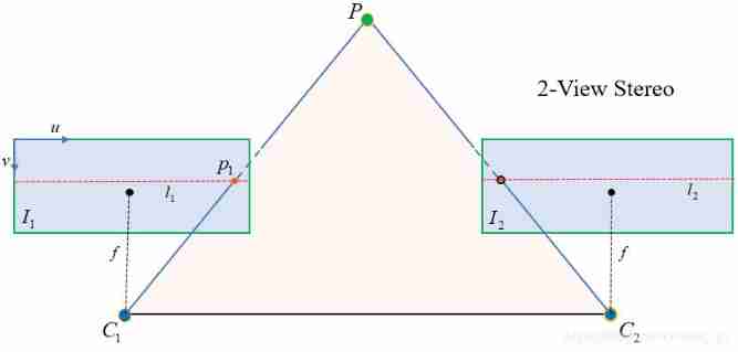

chart 3 Fusiello Epipolar correction In particular , The first step is to rotate the camera so that the image plane is coplanar and parallel to the camera baseline , It's actually redefining a camera coordinate system , So let's first look at how the new camera coordinate system is designed ：

1. First of all $X$ Axis , Obviously, it should be parallel to the camera baseline , To make the image plane parallel to the camera baseline , therefore $X$ The axis base vector is $r_x=(C_2-C_1)/||C_2-C_1||$.
2. The second is $Y$ Axis , It is and $X$ Axis orthogonal , You can set an arbitrary unit vector $k$, Give Way Y Axis and $X$ Axes and vectors $k$ orthogonal , therefore $Y$ The base vector of the axis is $r_y=k\times r_x$. About this $k$, Theoretically, anything can , However, we hope that the range of the image in the new coordinate system is consistent with that of the original image , So try to choose the old $Y$ The approximate orientation of the axis , stay Fusiello In law ,$k$ For the old $Z$ The unit vector represented by the axis .
3. And finally $Z$ Axis ,$X$ and $Y$ After the axis is determined ,$Z$ The basis vector of the axis can be obtained by the cross multiplication of the two based on the right-hand rule ：$r_z=r_x\times r_y$

Determine the new coordinate system 3 Base vectors , You can determine the new rotation matrix
$$R_n=\left[\begin{array}{c}{r}_x^{\text{T}}\\ r_y^{\text{T}}\\ r_z^{\text{T}}\end{array}\right]$$

On this point , You can take a look at my previous blog Understand rotation matrix from the perspective of base transformation R.

The second step , Is to redesign the new internal parameter matrix $K_n$, Theoretically ,$K$ It can be set arbitrarily , But in order to be consistent with the old camera ,Fusiello What cannot be chosen is $K_n=(K_{left}+K_{right})/2$. And put the tilt factor $s$ Set to 0.

determine $K$ and $R$ after , We get a new projection matrix $M_n=K_n[R_n|-R_{n}C]$.

Next is the calibration process , The specific process is for new image pixels $p_n$, By transforming the matrix $T$ Calculate the pixels on the old image $p$：$p=T{p}_n$, Then the pixel value is obtained by bilinear interpolation and assigned to the new image . So the key is how to get the transformation matrix $T$.

For the moment , We rotated the camera and redefined the internal parameters , This transforms the rotation matrix $R\to R_n$ And internal parameter matrix $K\to K_n$, What hasn't changed is the center of the camera $C$. So we now have two sets of projection matrices, old and new
$$\begin{array}{rlrl}M& =K[R,-RC]& & =[Q|-QC]\\ M_n& =K_n[R_n,-R_{n}C]& & =[Q_n|-Q_{n}C]\end{array}$$

among ,$Q=KR,Q_n=K_n{R}_n$.

Suppose a point in space $P$, Its projection expressions under the new and old projection matrices are ：
$$\begin{array}{rlrl}\lambda p& =MP& & =[Q|-QC]P\\ {\lambda }_n{p}_n& =M_{n}P& & =[Q_n|-Q_{n}C]P\end{array}$$

Because equations are homogeneous expressions （$p=[u,v,1],P=[X,Y,Z,1]$）, therefore $\lambda$ Can be set to 1. The above formula is expanded to
$$\begin{array}{rl}p& =Q(P-C)\\ p_n& =Q_n(P-C)\end{array}$$

Available ：
$$p_n=Q_n{Q}^{-1}p$$

This is the conversion formula of old and new images , and $T=Q_n{Q}^{-1}$ That is, the transformation matrix .

For two cameras , According to the formula, the respective transformation matrix can be calculated $T_1,T_2$.

Advantages and disadvantages

Fusiello The principle of law is very simple , Low computational complexity , And can be highly parallel , It's a good algorithm .

But there are some disadvantages , It assigns the same internal parameters to the new camera , In fact, it is not reasonable for a dual camera system with a large angle , Pictured 3 Shown , Keep the position of the main point approximately equal to the position of the old main point , For the original image pair with large included angle , The overlap area is significantly reduced , This is what we don't want to see , And if you set different primary coordinates for two cameras （ Specifically, it is the main point $x$ coordinate ）, Then the situation can be improved , As shown in the figure below ：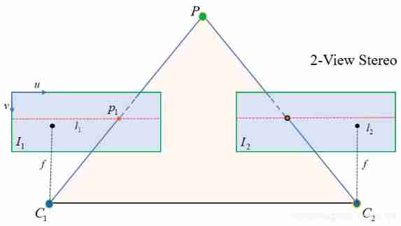

As for the adjustment amount of this main point , It has something to do with your camera design , If you are a two camera stereo system , Then it is suggested that you can follow Fusiello To design internal parameters , But set the width of the image as much as possible larger than the original width , Then visualize the results , Design interactive image clipping , After the clipping range is determined, the new principal point coordinates can be obtained . Because the binocular structure is fixed , So you just need to adjust once , If you don't move the structure, you don't have to adjust it .

That's all for today , If you have any questions, you can leave a message in the message area ！

About Fusiello Website of France , You can see Epipolar Rectification. by Andrea
Fusiello

The following is a pseudocode provided by the author , It's really simple , There is no need for me to do it again
https://homepages.inf.ed.ac.uk/rbf/CVonline/LOCAL_COPIES/FUSIELLO2/node5.html

Bye, everyone ！ Like collection and attention ！