当前位置:网站首页>How to optimize the deep learning model to improve the reasoning speed
How to optimize the deep learning model to improve the reasoning speed
2022-07-27 08:53:00 【DeepDriving】
Link to the original text :https://www.thinkautonomous.ai/blog/?p=deep-learning-optimization
Introduction
In deep learning , Inference refers to a forward propagation process of neural network , That is to send the input data into the neural network , The process of getting output results from it . such as , We can do this by 3D The point cloud is sent into a point cloud classification network to determine the category of the frame point cloud .

Knowing the reasoning time in advance can help us better design the deep learning model , And optimize the performance of reasoning . such as , We can replace the standard convolution with separable convolution to reduce the amount of computation , You can also prune 、 Quantification and model freezing to reduce the amount of calculation , These optimization techniques can reduce a lot of reasoning time . This article will briefly introduce these technologies .
How to calculate the reasoning time of the model
To understand how to optimize neural networks , We must have an indicator , Usually, this indicator is reasoning time , Reasoning time refers to the time required for the neural network to perform a forward propagation . Usually, we use the number of reasoning that the model can perform in one second to express the reasoning speed of the model , Unit use fps Express . Suppose the time required for model reasoning is 0.1s, Then its reasoning speed can be expressed as 1/0.1=10fps.
To measure the reasoning time of the model , We first need to understand 3 A concept : FLOPs, FLOPS, and MACs.
FLOPs
To measure the reasoning time of the model , We can calculate the total number of calculation operations that the model must perform . Put forward the term here
FLOP(Floating Point Operation), Floating point operation , These operations include addition 、 reduce 、 ride 、 Except for and any other operations related to floating-point numbers . A model ofFLOPsAll for this modelFLOPThe sum of the , This value can tell us the complexity of the model .FLOPS
FLOPSyesFloating Point Operations per SecondAbbreviation , Represents the number of floating-point operations that can be performed per second . This index can be used to measure the performance of the computing platform we use , The greater the value , It indicates that the more floating-point operands can be executed per second on this computing platform , Then the faster the reasoning speed of the model .MACs
MACsyesMultiply-Accumulate ComputationsAbbreviation . onceMACOperation means that an addition and a multiplication operation are performed , It is equivalent to doing two floating-point operations , So there is1 MAC = 2 FLOPS.
After understanding the above concepts , We naturally think of , If you want to make the deep learning model run faster , So we have two options :
Reduce
FLOPsvalue ;Improve... On the computing platform
FLOPSvalue .
For a specific computing platform , We cannot change its computing power , So if you want to achieve your goal , Then we need to optimize our model , Adopt certain technology to reduce the FLOPs value .
How to calculate the model FLOPs value
We take the following model as an example to introduce how to calculate the model FLOPs value , The model is a pair of MNIST A model for classification of handwritten digital data sets :
- The input data is
28x28x1The gray image ; - 2 Convolution layers , Each convolution layer contains 5 Size is
3x3Convolution kernel ; - A full connectivity layer , contain 128 Neurons ;
- A full connectivity layer , contain 10 Neurons , They represent from 0 To 9 Within the scope of 10 Categories ;

Calculation model FLOPs The formula for the value is as follows :
Convolution layer :
FLOPs = 2 * Number of convolution nuclei * Convolution kernel size * Output sizeamong , Output size =( Enter dimensions - Convolution kernel size ) + 1
Fully connected layer :
FLOPs = 2 * Enter dimensions * Output size
According to the above calculation method , We can calculate the FLOPs value ,
The first 1 Convolution layers :
FLOPs value = 2x5x(3x3)x26x26 = 60,840 FLOPs
The first 2 Convolution layers :
FLOPs value = 2x5x(3x3x5)x24x24 = 259,200 FLOPs
The first 1 All connection layers :
FLOPs value = 2x(24x24x5)x128 = 737,280 FLOPs
The first 2 All connection layers :
FLOPs value = 2x128x10 = 2,560 FLOPs
Then the whole model is all FLOPs value = 60,840 + 259,200 + 737,280 + 2,560 = 1,060,400 FLOPs.

Suppose the computing power of our computing platform is 1GFLOPS, Then it can be calculated that the time required for model reasoning on this computing platform is :
Reasoning time = 1,060,400 / 1,000,000,000 = 0.001s = 1ms
You can see , If we know about the computing platform FLOPS Value and model FLOPs Value is easy to calculate the reasoning time of the model .
How to optimize the model
Previously, I introduced how to calculate the reasoning time of the model , Let's get to the point , This paper introduces how to reduce the reasoning time of the model by optimizing the model . The methods of optimizing models are mainly divided into two types :
- Reduce model size ;
- Reduce computing operations ;
Reduce model size
The advantage of reducing the size of the model is that it can reduce the occupied storage space 、 Improve model loading speed 、 Improve reasoning speed, etc . Usually we can pass the following 3 Clock method reduces model size :
- quantitative
- Distillation of knowledge
- Weight sharing
quantitative
Quantization is the process of mapping values from a larger set to a smaller set . let me put it another way , We reduce the large continuous number , And replace them with smaller continuous numbers or even integers to achieve the purpose of quantification , For example, we can set the weight value 2.87950387409 Quantified as 2.9. We can quantify the weight and activation function , The result of quantization is to change the accuracy of the value , The most common is to 32 Bit floating point (FP32) or 16 Bit floating point (FP16) Quantified as 8 Bit integers (INT8) even to the extent that 4 Bit integers (INT4). The advantage of quantification is to reduce the amount of memory occupied by the model and reduce the computational complexity , However, due to reducing the weight of the model and the accuracy of the activation function , Usually, the reasoning accuracy of the quantized model will be reduced .
Weight sharing
Weight sharing refers to the sharing of weights between different neurons , By sharing , We can reduce some weight , Thus reducing the size of the model .
Distillation of knowledge
Knowledge distillation is a large-scale 、 Models with high accuracy (teacher) The acquired knowledge is transferred to simple structure 、 Models with lower computational costs (student) A method on . Knowledge distillation can be more vividly understood as the process of teachers teaching students : The teacher refines the knowledge he has learned , Then teach these knowledge to students , Although the knowledge learned by students is not as broad as that of teachers , But it is also deep in its essence .

Reduce computing operations
The main way to reduce computing operations is to use some more efficient 、 Operations with less computation are used to replace the original operations of the model . In this paper, 3 A way to reduce computational operations :
- Pooling (Pooling)
- Separable convolution (Separable Convolutions)
- Model pruning (Model Pruning)
Pooling
If you know something about deep learning , Then you must have heard of the maximum pooling operation and the average pooling operation , These pooling operations are designed to reduce computing operations . The pool layer is equivalent to a lower sampling layer , You can reduce the amount of parameters passed from one layer to another . Pooling layer is usually used after the convolution layer to retain spatial information , At the same time, reduce the number of parameters . The following figure is an example of a maximum pooling layer , The maximum pool operation is to retain the maximum value in the window and discard other values , So as to achieve the purpose of reducing parameters .

Separable convolution
Separable convolution is to divide the standard convolution layer into two convolution layers :depthwise Convolution sum pointwise Convolution .
depthwiseConvolution is also a common convolution , But it is different from the standard convolution . for instance , Suppose the input channel of the convolution layer is 4, The output channel is 8, The standard convolution is in 4 On input channels meanwhile Do convolution operation and take the result as an output channel , If you want to output 8 Two channels need to be 8 This convolution process ;depthwiseConvolution is , respectively, stay 4 Convolution operation on two channels , Then the result of each channel is used as an output channel , That is, the input is several channels , The output is just a few channels . In this case , The amount of computation for standard convolution to generate an output channel isdepthwiseConvolution generates an output channel calculation of 4 times .pointwiseConvolution is 1x1 Convolution of , Usually used indepthwiseAfter convolution , Used to deal withdepthwiseThe feature map generated by convolution integrates information in the depth direction .
use depthwise Convolution +pointwise The separable convolution of convolution replaces the standard convolution , It can significantly reduce the amount of calculation , Let's look at the example below :

In the diagram above ,depthwise Convolution +pointwise Convolution FLOPs The value is approximately 734KFLOPs. Let's look again at the calculation of standard convolution with the same parameters :

It can be seen that , Using standard convolution FLOPs The value is approximately 20MFLOPs, Is separable convolution 20 Many times . let me put it another way , In this case , Using separable convolution instead of standard convolution can improve the reasoning speed 20 Twice as many !
Model pruning
Pruning is a model compression technique , This method removes redundant network parameters while preserving the original accuracy of the network as much as possible to reduce the computational complexity of the model . In order to realize this technology , We first grade the whole model according to the importance of each neuron , Then delete the lower level neurons , So , We can set the connection of neurons to 0 Or set the weight to 0 To delete a neuron . By model pruning , We can get smaller 、 Reasoning is faster 、 The model with the least loss of reasoning accuracy .

Conclusion
Model optimization is a complex problem , As the saying goes, you can't have both fish and bear's paw . Although we can optimize the model through some methods to improve the reasoning speed , But doing so will inevitably bring the loss of accuracy , So we must balance speed and accuracy , Choose the best for 、 The most reasonable way to optimize the model .
Welcome to my official account. 【DeepDriving】, I will share computer vision from time to time 、 machine learning 、 Deep learning 、 Driverless and other fields .

边栏推荐
- Unity3d 2021 software installation package download and installation tutorial
- Day5 - Flame restful request response and Sqlalchemy Foundation
- Test picture
- Matlab solves differential algebraic equations (DAE)
- New year's goals! The code is more standardized!
- 数智革新
- VS Code中#include报错(新建的头文件)
- 【渗透测试工具分享】【dnslog服务器搭建指导】
- “蔚来杯“2022牛客暑期多校训练营1
- “寻源到结算“与“采购到付款“两者有什么不同或相似之处?
猜你喜欢

General Administration of Customs: the import of such products is suspended
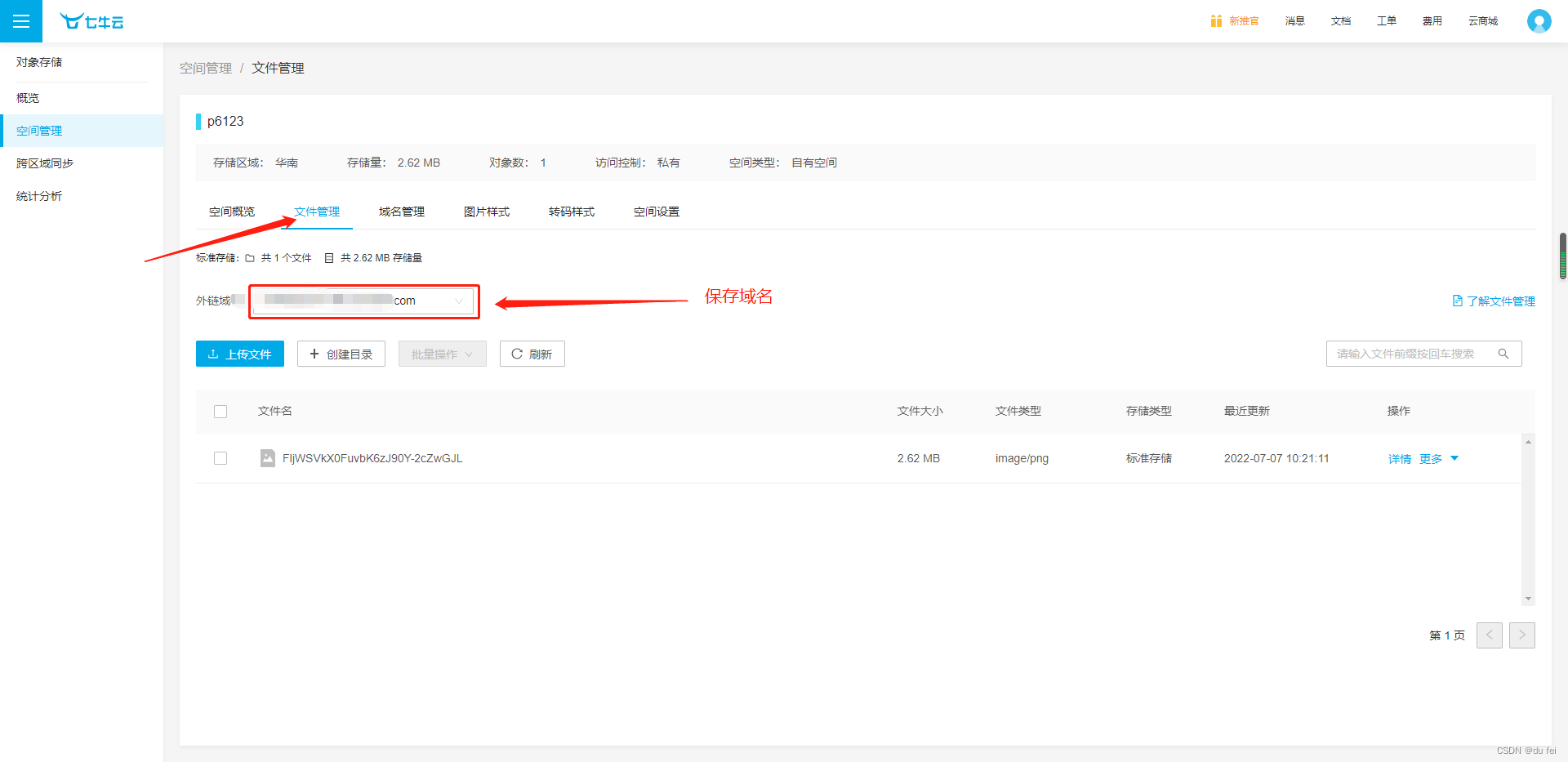
How to upload qiniu cloud

被三星和台积电挤压的Intel终放下身段,为中国芯片定制芯片工艺
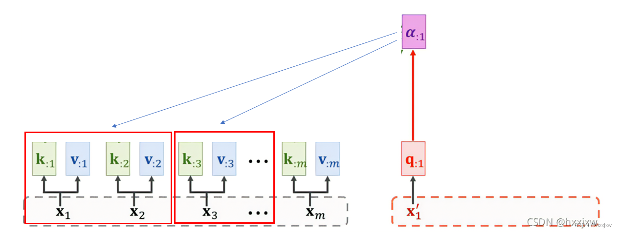
PVT的spatial reduction attention(SRA)

Mmrotate trains its dataset from scratch
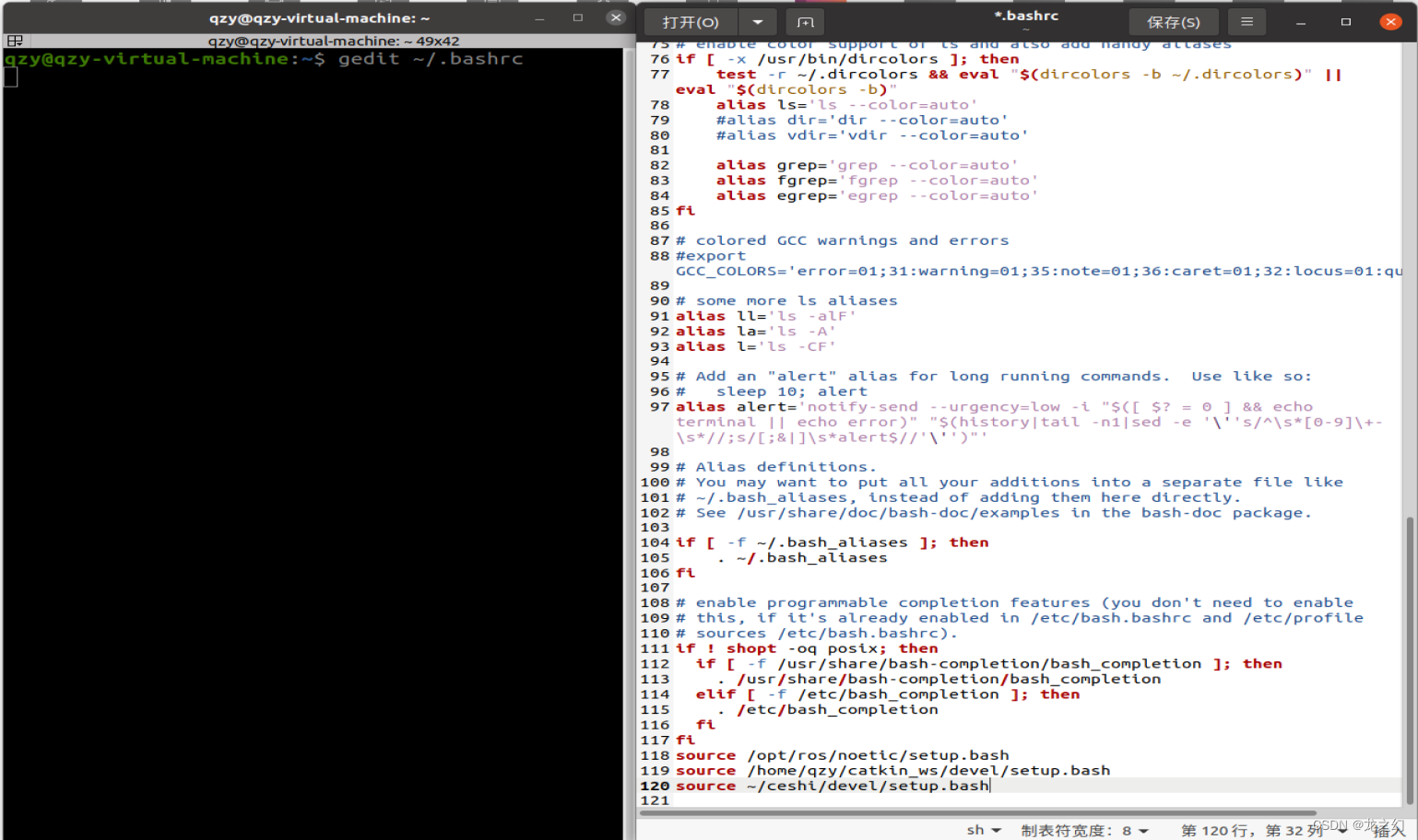
永久设置source的方法

Redis network IO

Cache consistency and memory barrier

Network IO summary

4279. 笛卡尔树
随机推荐
HUAWEI 机试题:字符串变换最小字符串 js
General Administration of Customs: the import of such products is suspended
Deep understanding of Kalman filter (3): multidimensional Kalman filter
JS检测客户端软件是否安装
[interprocess communication IPC] - semaphore learning
杭州电子商务研究院发布“数字化存在”新名词解释
Pass parameters and returned responses of flask
4279. Cartesian tree
2036: [Blue Bridge Cup 2022 preliminary] statistical submatrix (two-dimensional prefix sum, one-dimensional prefix sum)
Arm system call exception assembly
tensorflow包tf.keras模块构建和训练深度学习模型
[nonebot2] several simple robot modules (Yiyan + rainbow fart + 60s per day)
ROS2安装时出现Connection failed [IP: 91.189.91.39 80]
Network IO summary
Minio installation and use
Flask request data acquisition and response
HUAWEI 机试题:火星文计算 js
永久设置source的方法
Digital intelligence innovation
NIO示例