当前位置:网站首页>动手学深度学习_LeNet
动手学深度学习_LeNet
2022-08-04 11:36:00 【CV小Rookie】
LeNet 是最早发布的卷积神经网络之一,因其在计算机视觉任务中的高效性能而受到广泛关注。
没听说过也不要紧,对 MINIST 肯定不陌生,MNIST 数据集就是 LeNet 为了识别的目标。
当时,LeNet取得了与支持向量机(support vector machines)性能相媲美的成果,成为监督学习的主流方法
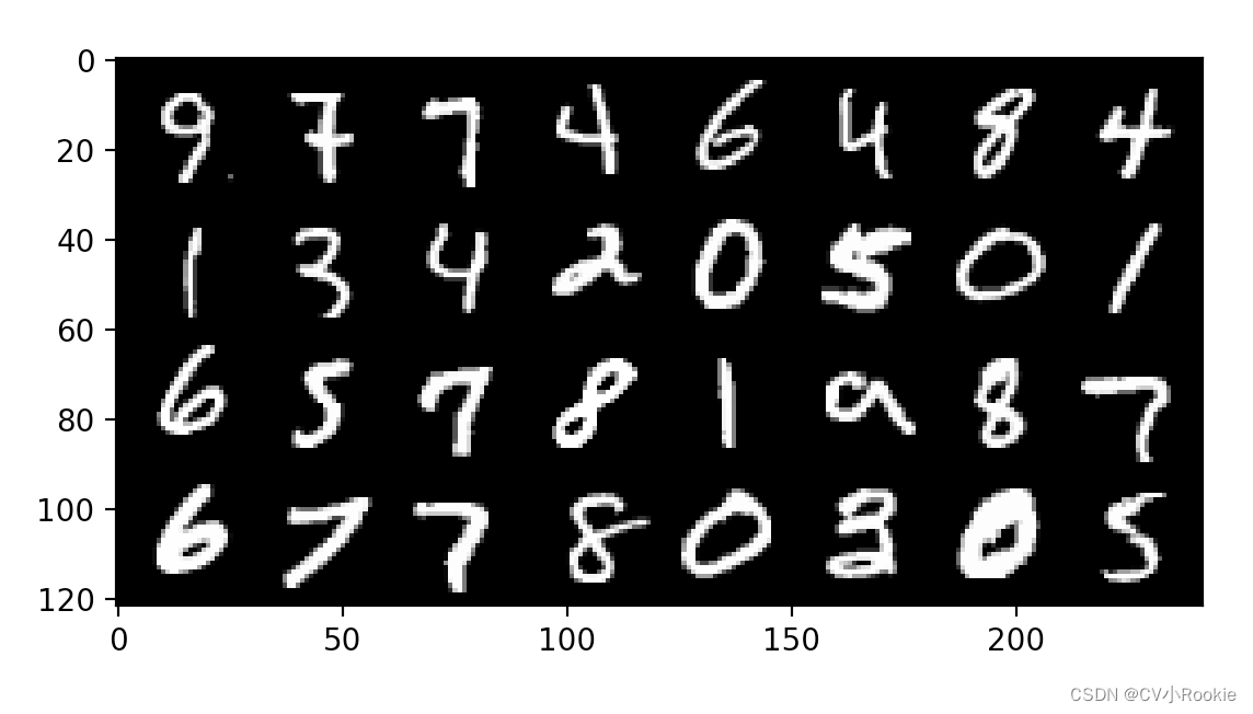
MNIST
简单介绍一下,MNIST 数据集共有 7w 张图片,其中 6w 用于训练,1w 用于测试。每张图像是 [email protected]*28 的黑白图像。
# 定义运行线程数
def get_dataloader_workers():  #@save
    """使用4个进程来读取数据"""
    return 4
# 下载MNIST数据集,然后将其加载到内存中
def load_data_mnist(batch_size, resize=None):  #@save
    trans = [transforms.ToTensor()]
    if resize:
        trans.insert(0, transforms.Resize(resize))
    trans = transforms.Compose(trans)
    mnist_train = torchvision.datasets.MNIST(root="../data", train=True, transform=trans, download=True)
    mnist_test = torchvision.datasets.MNIST(root="../data", train=False, transform=trans, download=True)
    return (data.DataLoader(mnist_train, batch_size, shuffle=True, num_workers=get_dataloader_workers()),
            data.DataLoader(mnist_test, batch_size, shuffle=False, num_workers=get_dataloader_workers()))
LeNet
LeNet有两个部分组成,前面的卷积模块和后面的全联接模块。卷积用来提取特征,全联接用来映射最后输出进行分类。
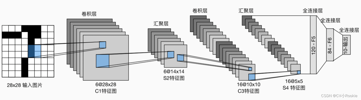
每个卷积块中的基本单元是一个卷积层、一个sigmoid激活函数和 average pooling 层(虽然 ReLU 和 max pooling 更有效,但它们在20世纪90年代还没有出现)。每个卷积层使用5×5卷积核和一个sigmoid激活函数。这些层将输入映射到多个二维特征输出,通常同时增加通道的数量。第一卷积层有6个输出通道,而第二个卷积层有16个输出通道。每个2×2池操作(stride为2)通过空间下采样将维数减少4倍。卷积的输出形状由批量大小、通道数、高度、宽度决定。
为了将卷积块的输出传递给稠密块,我们必须在小批量中展平每个样本。换言之,我们将这个四维输入转换成全连接层所期望的二维输入。这里的二维表示的第一个维度索引小批量中的样本,第二个维度给出每个样本的平面向量表示。LeNet的稠密块有三个全连接层,分别有120、84和10个输出。因为我们在执行分类任务,所以输出层的10维对应于最后输出结果的数量。
直接上代码!
# 作者 :CV小Rookie
# 创建时间: 2022/8/3 20:45
# 文件名: train.py
import torch
from torch import nn
from d2l import torch as d2l
from download_datas import *

def get_default_device():
    if torch.cuda.is_available() :
        return 'cuda'
    elif getattr (torch.backends, 'mps', None) is not None and torch.backends.mps.is_available():
        return 'mps'
    else:
        return 'cpu'
device = get_default_device()

net = nn.Sequential(
    nn.Conv2d(1, 6, kernel_size=5, padding=2), nn.Sigmoid(),
    nn.AvgPool2d(kernel_size=2, stride=2), #
    nn.Conv2d(6, 16, kernel_size=5), nn.Sigmoid(),
    nn.AvgPool2d(kernel_size=2, stride=2),
    nn.Flatten(),
    nn.Linear(16 * 5 * 5, 120), nn.Sigmoid(),
    nn.Linear(120, 84), nn.Sigmoid(),
    nn.Linear(84, 10))

# X = torch.rand(size=(1, 1, 28, 28), dtype=torch.float32)
# for layer in net:
#     X = layer(X)
#     print(layer.__class__.__name__,'output shape: \t',X.shape)
print(net)

batch_size = 256
train_iter, test_iter = load_data_mnist(batch_size=batch_size)
# train_iter, test_iter = load_data_fashion_mnist(batch_size=batch_size)

def evaluate_accuracy_gpu(net, data_iter, device=None): #@save
    """使用GPU计算模型在数据集上的精度"""
    if isinstance(net, nn.Module):
        net.eval()  # 设置为评估模式
        if not device:
            device = next(iter(net.parameters())).device
    # 正确预测的数量,总预测的数量
    metric = d2l.Accumulator(2)
    with torch.no_grad():
        for X, y in data_iter:
            if isinstance(X, list):
                # BERT微调所需的(之后将介绍)
                X = [x.to(device) for x in X]
            else:
                X = X.to(device)
            y = y.to(device)
            metric.add(d2l.accuracy(net(X), y), y.numel())
    return metric[0] / metric[1]

def train(net, train_iter, test_iter, num_epochs, lr, device):
    def init_weights(m):
        if type(m) == nn.Linear or type(m) == nn.Conv2d:
            nn.init.xavier_uniform_(m.weight)
    net.apply(init_weights)
    print('training on', device)
    net.to(device)
    optimizer = torch.optim.SGD(net.parameters(), lr=lr)
    loss = nn.CrossEntropyLoss()
    animator = d2l.Animator(xlabel='epoch', xlim=[1, num_epochs],
                            legend=['train loss', 'train acc', 'test acc'])
    timer, num_batches = d2l.Timer(), len(train_iter)
    for epoch in range(num_epochs):
        # 训练损失之和,训练准确率之和,样本数
        metric = d2l.Accumulator(3)
        net.train()
        for i, (X, y) in enumerate(train_iter):
            timer.start()
            optimizer.zero_grad()
            X, y = X.to(device), y.to(device)
            y_hat = net(X)
            l = loss(y_hat, y)
            l.backward()
            optimizer.step()
            with torch.no_grad():
                metric.add(l * X.shape[0], d2l.accuracy(y_hat, y), X.shape[0])
            timer.stop()
            train_l = metric[0] / metric[2]
            train_acc = metric[1] / metric[2]
            if (i + 1) % (num_batches // 5) == 0 or i == num_batches - 1:
                animator.add(epoch + (i + 1) / num_batches,
                             (train_l, train_acc, None))
        test_acc = evaluate_accuracy_gpu(net, test_iter)
        animator.add(epoch + 1, (None, None, test_acc))
        torch.save(net.state_dict(), "module-{0}.pth".format(epoch))
    print(f'loss {train_l:.3f}, train acc {train_acc:.3f}, '
          f'test acc {test_acc:.3f}')
    print(f'{metric[2] * num_epochs / timer.sum():.1f} examples/sec '
          f'on {str(device)}')

lr, num_epochs = 0.9, 10
train(net, train_iter, test_iter, num_epochs, lr, device)以[email protected]输入为例
Conv2d output shape: torch.Size([1, 6, 28, 28])
Sigmoid output shape: torch.Size([1, 6, 28, 28])
AvgPool2d output shape: torch.Size([1, 6, 14, 14])
Conv2d output shape: torch.Size([1, 16, 10, 10])
Sigmoid output shape: torch.Size([1, 16, 10, 10])
AvgPool2d output shape: torch.Size([1, 16, 5, 5])
Flatten output shape: torch.Size([1, 400])
Linear output shape: torch.Size([1, 120])
Sigmoid output shape: torch.Size([1, 120])
Linear output shape: torch.Size([1, 84])
Sigmoid output shape: torch.Size([1, 84])
Linear output shape: torch.Size([1, 10])
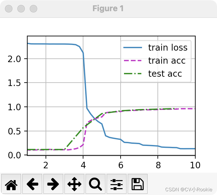
loss 0.131, train acc 0.961, test acc 0.966
边栏推荐
- Doing Homework HDU - 1074
- cat /proc/kallsyms found that the kernel symbol table values are all 0
- MySQL索引原理以及SQL优化
- 【目标检测】YOLOv4特征提取网络——CSPDarkNet53结构解析及PyTorch实现
- ESP8266-Arduino编程实例-MQ3酒精传感器驱动
- Rust 从入门到精通04-变量
- ping的原理
- Leetcode brush questions - 543. Diameter of binary trees, 617. Merging binary trees (recursive solution)
- SkiaSharp 之 WPF 自绘 粒子花园(案例版)
- yolov5——detect.py代码【注释、详解、使用教程】
猜你喜欢
Leetcode刷题——构造二叉树(105. 从前序与中序遍历序列构造二叉树、106. 从中序与后序遍历序列构造二叉树)
God Space - the world's first Web3.0-based art agreement creative platform, broadening the boundaries of multi-art integration
上帝空间——全球首个基于Web3.0的艺术协议创意平台,拓宽多元艺术融合边界
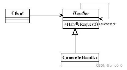
职责链模式(responsibilitychain)
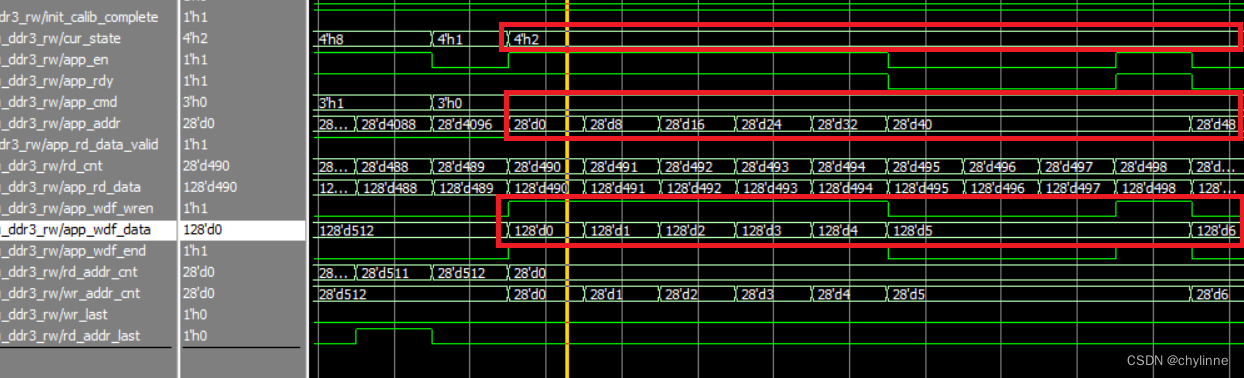
The use of DDR3 (Naive) in Xilinx VIVADO (3) simulation test
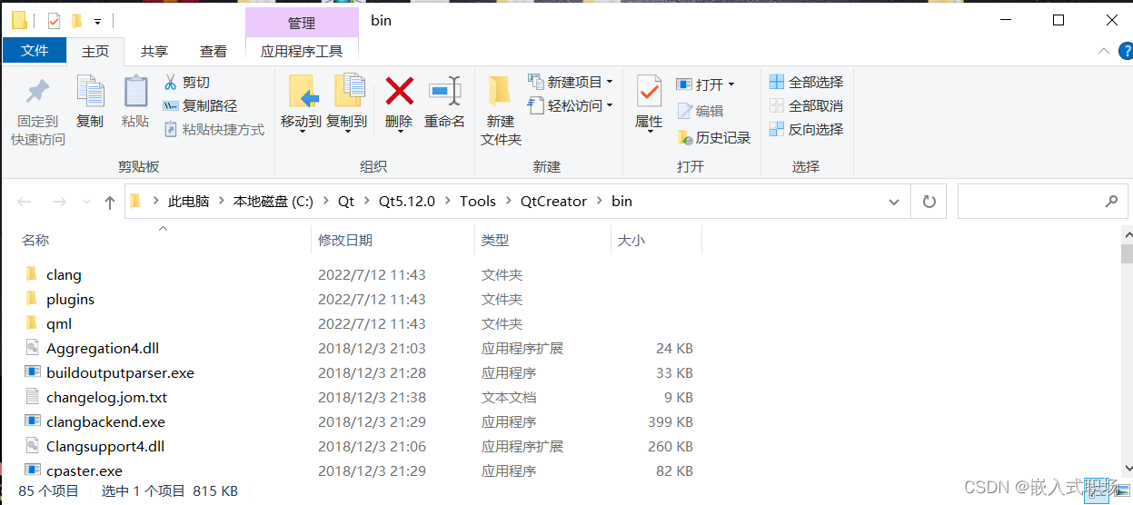
【Qt】解决 “由于找不到Qt5Cored.dll,无法继续执行代码”(亲测有效)

技术干货 | 用零信任保护代码安全
【LeetCode】700.二叉搜索树
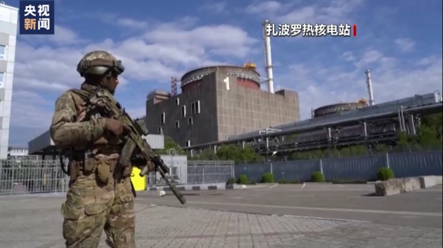
国际原子能机构总干事警告称扎波罗热核电站安全形势已“完全失控”
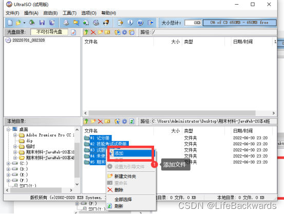
光盘刻录步骤
随机推荐
面试蚂蚁(P7)竟被MySQL难倒,奋发图强后二次面试入职蚂蚁金服
能力更强,医疗单据识别+医疗知识库校验
单调栈一些题目练习
涨姿势了!原来这才是多线程正确实现方式
企业应当实施的5个云安全管理策略
使用.NET简单实现一个Redis的高性能克隆版(二)
力扣解法汇总1403-非递增顺序的最小子序列
Mysql——》类型转换符binary
SchedulX V1.5.0发布,提供快速压测、对象存储等全新功能!
Mysql高级篇学习总结13:多表连接查询语句优化方法(带join语句)
终于有人把分布式机器学习讲明白了
入门MySql表的增删查改
MySql数据库入门的基本操作
AI 助力双碳目标:让每一度电都是我们优化的
萌宠来袭,如何让“吸猫撸狗”更有保障?
ESP8266-Arduino编程实例-APDS-9930环境光和趋近感器驱动
Leetcode刷题——构造二叉树(105. 从前序与中序遍历序列构造二叉树、106. 从中序与后序遍历序列构造二叉树)
【目标检测】------yolo:xml和txt文件相互转化
国际原子能机构总干事警告称扎波罗热核电站安全形势已“完全失控”
POJ1094Sorting It All Out题解