当前位置:网站首页>【推荐系统基础】正负样本采样和构造
【推荐系统基础】正负样本采样和构造
2022-07-07 21:53:00 【山顶夕景】
文章目录
一、回顾word2vec中的负采样
- word2vec中的负采样:CBOW或者skip-gram这类模型的训练,在当词表规模较大且计算资源有限时,这类多分类模型会因为输出层(softmax)概率的归一化计算效率的影响,以免训练龟速。
- 而负采样提供了另一个角度:给定当前词与上下文,任务是最大化两者的共现概率。
也即将多分类问题简化为:针对(w, c)的二分类问题(即共现or不共现),从而避免了大词表上的归一化复杂计算量。
如 P ( D = 1 ∣ w , c ) P(D=1 \mid w, c) P(D=1∣w,c)表示c和w共现的概率 P ( D = 1 ∣ w , c ) = σ ( v w ⋅ v c ′ ) P(D=1 \mid w, c)=\sigma\left(v_{w} \cdot v_{c}^{\prime}\right) P(D=1∣w,c)=σ(vw⋅vc′)
1.1 滑动窗口
为了得到每个单词的高质量稠密embedding(相似上下文的单词的vector应该相似),word2vec是通过一个滑动窗口的滑动,同时计算 P ( w t + j ∣ w t ) P\left(w_{t+j} \mid w_{t}\right) P(wt+j∣wt)。下面就是一个栗子,window_size=2。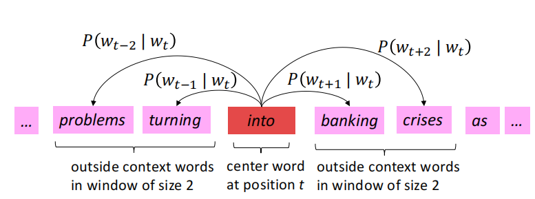
1.2 目标函数
(1)一开始我们将刚才得到的一坨 P ( w t + j ∣ w t ) P\left(w_{t+j} \mid w_{t}\right) P(wt+j∣wt)相乘,并且是对于每个t,所以有2个累乘:
(2)因为一般我们是最小化目标函数,所以进行了取log和负平均的操作,修改后的目标函数: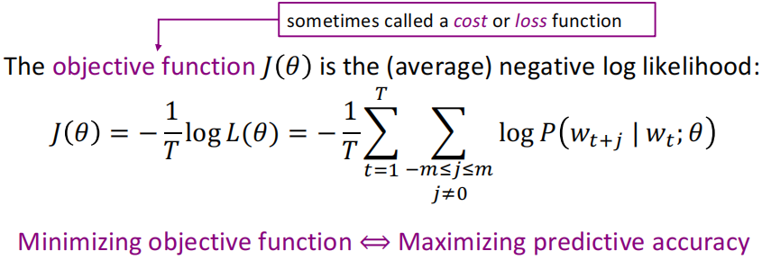
为了求出上面损失函数最里面的概率 P ( w t + j ∣ w t ; θ ) P\left(w_{t+j} \mid w_{t} ; \theta\right) P(wt+j∣wt;θ),对于每个单词都用2个vector表示:
- 当w是中心词时,表示为 v w v_w vw
- 当w是上下文词时,表示为 u w u_w uw
但是为啥要用两个vector表示每个单词呢——更容易optimization。
1.3 预测函数
所以对于一个中心词c和一个上下文次c有: P ( o ∣ c ) = exp ( u o T v c ) ∑ w ∈ V exp ( u w T v c ) P(o \mid c)=\frac{\exp \left(u_{o}^{T} v_{c}\right)}{\sum_{w \in V} \exp \left(u_{w}^{T} v_{c}\right)} P(o∣c)=∑w∈Vexp(uwTvc)exp(uoTvc)将任意值 x i x_i xi映射到概率分布中,即如下: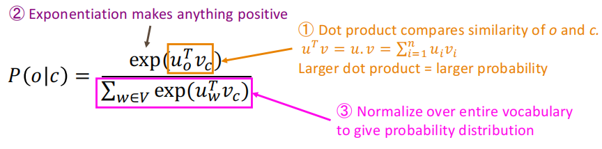
分子的点积用来表示o和c之间相似程度,分母这坨东西就是基于整个词表,给出归一化后的概率分布。
二、word2vec中的负采样实现
下面是基于负采样的skip-gram模型,对于每个需要训练的正样本数据,需要按照某个负采样概率生成对应的负样本,有两种实现方法:
- 在构建数据时就生成对应的负样本,在训练模型时就不用再构建负样本了,但是缺点是每次迭代使用的是相同的负样本,缺乏多样性;
- 下面使用的是在训练时构造对应的负样本,利用
SGNSDataset中的collate_fn实现,对batch内样本进行负采样。
import torch
import torch.nn as nn
import torch.nn.functional as F
import torch.optim as optim
from torch.utils.data import Dataset
from torch.nn.utils.rnn import pad_sequence
from tqdm.auto import tqdm
from utils import BOS_TOKEN, EOS_TOKEN, PAD_TOKEN
from utils import load_reuters, save_pretrained, get_loader, init_weights

class SGNSDataset(Dataset):
    def __init__(self, corpus, vocab, context_size=2, n_negatives=5, ns_dist=None):
        self.data = []
        self.bos = vocab[BOS_TOKEN]
        self.eos = vocab[EOS_TOKEN]
        self.pad = vocab[PAD_TOKEN]
        for sentence in tqdm(corpus, desc="Dataset Construction"):
            sentence = [self.bos] + sentence + [self.eos]
            for i in range(1, len(sentence)-1):
                # 模型输入:(w, context) ;输出为0/1,表示context是否为负样本
                w = sentence[i]
                left_context_index = max(0, i - context_size)
                right_context_index = min(len(sentence), i + context_size)
                context = sentence[left_context_index:i] + sentence[i+1:right_context_index+1]
                context += [self.pad] * (2 * context_size - len(context))
                self.data.append((w, context))

        # 负样本数量
        self.n_negatives = n_negatives
        # 负采样分布:若参数ns_dist为None,则使用uniform分布
        self.ns_dist = ns_dist if ns_dist is not None else torch.ones(len(vocab))

    def __len__(self):
        return len(self.data)

    def __getitem__(self, i):
        return self.data[i]

    def collate_fn(self, examples):
        words = torch.tensor([ex[0] for ex in examples], dtype=torch.long)
        contexts = torch.tensor([ex[1] for ex in examples], dtype=torch.long)
        batch_size, context_size = contexts.shape
        neg_contexts = []
        # 对batch内的样本分别进行负采样
        for i in range(batch_size):
            # 保证负样本不包含当前样本中的context
            ns_dist = self.ns_dist.index_fill(0, contexts[i], .0)
            neg_contexts.append(torch.multinomial(ns_dist, self.n_negatives * context_size, replacement=True))
        neg_contexts = torch.stack(neg_contexts, dim=0)
        return words, contexts, neg_contexts

class SGNSModel(nn.Module):
    def __init__(self, vocab_size, embedding_dim):
        super(SGNSModel, self).__init__()
        # 词嵌入
        self.w_embeddings = nn.Embedding(vocab_size, embedding_dim)
        # 上下文嵌入
        self.c_embeddings = nn.Embedding(vocab_size, embedding_dim)

    def forward_w(self, words):
        w_embeds = self.w_embeddings(words)
        return w_embeds

    def forward_c(self, contexts):
        c_embeds = self.c_embeddings(contexts)
        return c_embeds


def get_unigram_distribution(corpus, vocab_size):
    # 从给定语料中统计unigram概率分布
    token_counts = torch.tensor([0] * vocab_size)
    total_count = 0
    for sentence in corpus:
        total_count += len(sentence)
        for token in sentence:
            token_counts[token] += 1
    unigram_dist = torch.div(token_counts.float(), total_count)
    return unigram_dist

embedding_dim = 64
context_size = 2
hidden_dim = 128
batch_size = 1024
num_epoch = 10
n_negatives = 10

# 读取文本数据
corpus, vocab = load_reuters()
# 计算unigram概率分布
unigram_dist = get_unigram_distribution(corpus, len(vocab))
# 根据unigram分布计算负采样分布: p(w)**0.75
negative_sampling_dist = unigram_dist ** 0.75
negative_sampling_dist /= negative_sampling_dist.sum()
# 构建SGNS训练数据集
dataset = SGNSDataset(
    corpus,
    vocab,
    context_size=context_size,
    n_negatives=n_negatives,
    ns_dist=negative_sampling_dist
)
data_loader = get_loader(dataset, batch_size)

device = torch.device('cuda' if torch.cuda.is_available() else 'cpu')
model = SGNSModel(len(vocab), embedding_dim)
model.to(device)
optimizer = optim.Adam(model.parameters(), lr=0.001)

model.train()
for epoch in range(num_epoch):
    total_loss = 0
    for batch in tqdm(data_loader, desc=f"Training Epoch {
      epoch}"):
        words, contexts, neg_contexts = [x.to(device) for x in batch]
        optimizer.zero_grad()
        batch_size = words.shape[0]
        # 提取batch内词、上下文以及负样本的向量表示
        word_embeds = model.forward_w(words).unsqueeze(dim=2)
        context_embeds = model.forward_c(contexts)
        neg_context_embeds = model.forward_c(neg_contexts)
        # 正样本的分类(对数)似然
        context_loss = F.logsigmoid(torch.bmm(context_embeds, word_embeds).squeeze(dim=2))
        context_loss = context_loss.mean(dim=1)
        # 负样本的分类(对数)似然
        neg_context_loss = F.logsigmoid(torch.bmm(neg_context_embeds, word_embeds).squeeze(dim=2).neg())
        neg_context_loss = neg_context_loss.view(batch_size, -1, n_negatives).sum(dim=2)
        neg_context_loss = neg_context_loss.mean(dim=1)
        # 损失:负对数似然
        loss = -(context_loss + neg_context_loss).mean()
        loss.backward()
        optimizer.step()
        total_loss += loss.item()
    print(f"Loss: {
      total_loss:.2f}")

# 合并词嵌入矩阵与上下文嵌入矩阵,作为最终的预训练词向量
combined_embeds = model.w_embeddings.weight + model.c_embeddings.weight
save_pretrained(vocab, combined_embeds.data, "sgns.vec")
三、推荐系统中召回相关基础
召回模型训练与评估(对应的损失函数)
- Point-wise样本构造:BCE Loss
- Pair-wise样本构造:BPR Hinge Loss
- List-wise样本构造:softmax Loss
- 向量化召回:使用annoy
3.1 召回中的三种训练方式
召回中,一般的训练方式分为三种:point-wise、pair-wise、list-wise。在datawhale的RecHub中,用参数mode来指定训练方式,每一种不同的训练方式也对应不同的Loss。
对应的三种训练方式可以参考下图(3种),其中a表示user的embedding,b+表示正样本的embedding,b-表示负样本的embedding。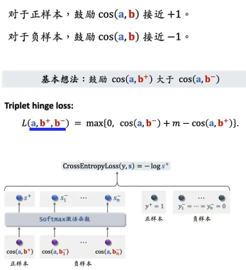
(1)Point wise (mode = 0)
思想:将召回视作二分类,独立看待每个正样本、。
对于一个召回模型:
- 输入二元组<User, Item>,
- 输出 P ( U s e r P(U s e r P(User, Item ) ) ), 表示 User 对 Item 的感兴趣程度。
- 训练目标为: 若物品为正样本, 输出应尽可能接近 1 , 负样本则输出尽可能接近 0 。 采用的 Loss 最常见的就是 BCELoss(Binary Cross Entropy Loss)。
(2)Pair wise (mode = 1)
思想:用户对正样本感兴趣的程度应该大于负样本。
对于一个召回模型:
- 输入三元组<User, ItemPositive, ItemNegative>,
- 输出兴趣得分 P ( P( P( User, ItemPositive ) , P ( ), P( ),P( User, ItemNegative ) ) ), 表示用户对正样本物品和负样 本物品的兴趣得分。
- 训练目标为:正样本的兴趣得分应尽可能大于负样本的兴趣得分。
torch-rechub框架中采用的 Loss 为 BPRLoss(Bayes Personalized Ranking Loss)。Loss 的公式这里放 一个公式, 详细可以参考【贝叶斯个性化排序(BPR)算法小结】(链接里的内容和下面的公式有些细微的差别, 但是思想是一 样的)
L o s s = 1 N ∑ N i i = 1 − log ( L o s s=\frac{1}{N} \sum^{N} i_{i=1}-\log ( Loss=N1∑Nii=1−log( sigmoid ( ( ( pos_score − - − neg_score ) ) )) ))
(3)List wise(mode = 2)
思想:思想同Pair wise,但是实现上不同。
对于一个召回模型:
- 输入 N + 2 \boldsymbol{N}+2 N+2 元 组 * \langle * User, ItemPositive, ItemNeg_1,…, ItemNeg_N * \rangle *;
- 输出用户对 1 个正样本和 N \mathrm{N} N 个负样本的兴趣得分。
- 训练目标为:对正样本的兴趣得分应该尽可能大于其他所有负样本的兴趣得分。
torch rechub框架中采用的 Loss 为 torch.nn.CrossEntropyLoss, 即对输出进行 Softmax 处理后取交叉熵。
PS: 这里的 List wise 方式容易和 Ranking 中的 List wise 混淆, 虽然二者名字一样, 但 ranking 的 List wise 考虑了样本之间的顺序关系。例如 ranking 中会考虑 MAP、NDCP 等考虑顺序的指标作为评价指标, 而 Matching 中的 List wise 没有考虑顺序。
四、推荐系统中的负采样
在模型训练中,需要提供正例(用户喜欢商品)和负例(用户不喜欢的商品)给模型,但是由于在实际推荐场景中数据收集的难度,一般很难获得非用户的显式反馈行为(如用户对item的评分等),但用户的隐式反馈信息(用户消费或者有交互过的item)是较容易得到的。
一般假设用户交互过的商品都是正例,并通过采样的方式,从用户未交互过的商品集中选择一部分作为负例。
负采样(Negative Sampling):从用户未交互商品集中基于一定策略进行负例选择的这一过程。
- DSSM召回的样本中:
- 正样本就是曝光给用户并且用户点击的item;
- 负样本:其实常见错误是直接使用曝光并且没被user点击的item,但是会导致SSB(sample selection bias)样本选择偏差问题——因为召回在线时时从全量候选item中召回,而不是从有曝光的item中召回。
DSSM原始论文里的做法:只有正样本, 记为 D + D^{+} D+, 对于用户 u 1 u_{1} u1, 其正样本就是其点击过的 item, 负样本则是随机从 D + D^{+} D+(不包含 u 1 u_{1} u1 点击过的item) 中随机选择4个item作为负样本。
4.1 负样本构造的6个常用方法
(1)曝光未点击数据
如果只用这个,会导致BBS问题,也要看场景。
(2)全局随机选择负例
从原始的全局物料库中,随机抽取作为召回或者粗排的负样本。
(3)Batch内随机选择负例
训练时在同一个batch中,在除了正例之外的其他item,选择构造负例,一定程度解决SSB问题。
(4)曝光数据中随机选择负例
(5)基于Popularity随机选择负例
越流行的item,如果没被用户点击看过,则更可能对于该用户来说是一个真实的负例。
(6)基于Hard选择负例
作为easy negative 的一种补充,hard negative是比较难的负样本,即匹配度适中的,用户可能喜欢也可能不喜欢——但实际上是用户不喜欢的!可以参考Airbnb筛选Hard负例的尝试(hard例给模型带来的loss和信息多)。
业务逻辑选取(以airbnb为例)
- i 增加与正样本同城的房间作为负样本,增强了正负样本在地域上的相似性,加大了模型的学习难度
- ii 增加“被房主拒绝”作为负样本,增强了正负样本在“匹配用户兴趣爱好”上的相似性,加大了模型的学习难度
模型挖掘
- EBR与百度Mobius的做法极其相似,都是用上一版本的召回模型筛选出"没那么相似"的<user,doc>对,作为额外负样本,训练下一版本召回模型。
- EBR的做法是:采用上一版模型召回位置在101~500上的item作为hard negative(负样本还是以easy negative为主,文章中经验值是easy:hard=100:1)
Reference
[1] Word2Vec中为什么使用负采样?
[2] 一文读懂推荐系统负采样
[3] 负采样Negative Sampling
[4] 【机器学习】推荐算法正负样本选择方法调研总结
[5] CTR预估模型中的正负样本定义、选择和比例控制
[6] 关于推荐系统中召回模块建模采样方式的讨论
[7] 推荐系统(四)—— 负采样
边栏推荐
猜你喜欢
Learn about scratch
Traduction gratuite en un clic de plus de 300 pages de documents PDF
Kubectl 好用的命令行工具:oh-my-zsh 技巧和窍门

Aitm3.0005 smoke toxicity test
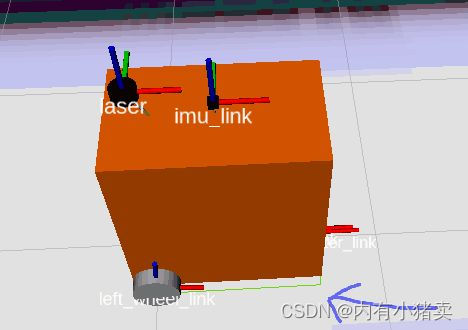
Laser slam learning (2d/3d, partial practice)
Ora-01741 and ora-01704

串联二极管,提高耐压
Connect diodes in series to improve voltage withstand
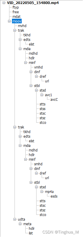
An example analysis of MP4 file format parsing
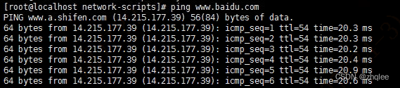
ping报错:未知的名称或服务
随机推荐
Go time package common functions
Orthodontic precautions (continuously updated)
Connect diodes in series to improve voltage withstand
一份假Offer如何盗走了「Axie infinity」5.4亿美元?
平衡二叉樹【AVL樹】——插入、删除
SQL uses the in keyword to query multiple fields
Dependency injection
Flash download setup
HDU - 1260 Tickets(线性DP)
Ping error: unknown name or service
Binary sort tree [BST] - create, find, delete, output
DataGuard active / standby cleanup archive settings
Come on, brother
[leetcode] 20. Valid brackets
Where are you going
C语言学习
Navicat connects Oracle
Take you hand in hand to build Eureka client with idea
[experiment sharing] log in to Cisco devices through the console port
Extract the file name under the folder under win