Shiyou's numerical analysis assignment

Want to make APP Same thing as WeChat , Can run small programs smoothly ？ | Experience will send you to Xinjiang 、 Huawei 、 Cherry keyboard ！>>>

It suddenly occurred to me that I could do numerical analysis , So I took my roommate's numerical analysis homework to practice , Write a blog to share . In fact, I'm a rookie who has complicated the program , There are many things that can be simplified , Because this novice has not finished other homework , I don't want to simplify , You can correct it by yourself .

---

Numerical analysis on computer

First of all, let me talk about my doubts , For the first question python How to achieve to ln(x) Call the derivative directly ？ Is it a direct derivative of a polynomial after Taylor expansion ？ The second question is to use Newton Iterative method , It is required to find out the range of the initial value of iteration in which the convergent solution can be obtained , If we use iterative program to implement it, it will be more troublesome , Is there a better way to solve it ？ I hope there is a God who can help me to leave a message , Thank you very much .

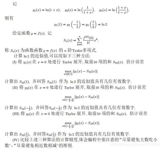
One 、 topic 1—— Approximate solution of logarithm

1. Title Description

** subject ：** There's a lot of laziness here , Just post the screenshot of the original question .

2.python Realization

Not much BB, The program is here ：

import numpy as np
from sympy import * # It is used in scientific calculation such as derivative integral 
import math as m

x = Symbol('x')#x  Variable 
t = Symbol('t')
y1 = 1/(1+x) # The formula 
y2 = -1/(1+x) # The formula 
y3 = 2/(1-x**2) # The formula 

def func(m):
    res = m
    for j in range(1,m):
        res *= j
    return res

def ln_Tyalor(y):
    Tl_expr = y * (t-x)
    for i in range(1, 10):
        fac = func(i+1)
        f_n = diff(y, x, i)
        Tl_expr += (f_n / fac)*(t-x)**(i+1)
    return Tl_expr.subs({
   
    x:0})

#print(ln_Tyalor(y1))
sexpr1 = ln_Tyalor(y1)
sexpr2 = ln_Tyalor(y2)
sexpr3 = ln_Tyalor(y3)
A = sexpr1.subs({
   
    t:1}).evalf()
B = sexpr2.subs({
   
    t:-1/2}).evalf()
C = sexpr3.subs({
   
    t:1/3}).evalf()
print('ln2 Value ：', m.log(2, m.e))
print(' equation ln(1+x) Of 10 The result of Taylor expansion is ：', A,'\n',' The estimated error is ：', abs(m.log(2, m.e)-A))
print(' equation ln(1/(1+x)) Of 10 The result of Taylor expansion is ：', B,'\n',' The estimated error is ：', abs(m.log(2, m.e)-B))
print(' equation ln((1+x)/(1-x)) Of 10 The result of Taylor expansion is ：', C,'\n',' The estimated error is ：', abs(m.log(2, m.e)-C))

3. Output results

ln2 Value ： 0.6931471805599453
 equation ln(1+x) Of 10 The result of Taylor expansion is ： 0.645634920634921 
  The estimated error is ： 0.0475122599250246
 equation ln(1/(1+x)) Of 10 The result of Taylor expansion is ： 0.693064856150793 
  The estimated error is ： 8.23244091517905e-5
 equation ln((1+x)/(1-x)) Of 10 The result of Taylor expansion is ： 0.693146047390827 
  The estimated error is ： 1.13316911820593e-6

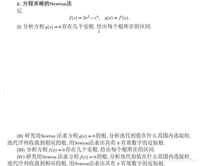
One 、 topic 2—— The root of an equation Newton Law

1. Title Description

** subject ：** Or the screenshots are convenient .

2.python Realization

This program is not well written , Because after writing ,exp（） Functions always report errors ： Integer data is not exp Object properties , I didn't realize my idea after I changed it , So be it , There's no time. , Let's do it ourselves .....

import numpy as np
from sympy import * # It is used in scientific calculation such as derivative integral 
import math as m

def f(x):
    return 3*x**2 - m.exp(x) # The equation has 3 A root , A preliminary estimate is that [-1,0],[0,1],[3,4]

def fdiff(x):
    return 6*x - m.exp(x)

def g(x):
    return 6*x - m.exp(x)# The equation has 3 A root , A preliminary estimate is that [0,1],[2,3]

def gdiff(x):
    return 6 - m.exp(x)

a = float(input(' Please enter the lower bound of the calculation interval a( floating-point ）: '))
b = float(input(' Please enter the upper bound of the calculation interval b( floating-point ）: '))
c = float(input(' Please enter the iteration initial value ( floating-point ）: '))
n = input(' Please enter the function to be solved ,f representative f(x),g representative g(x): ')

if n =='f':

    if f(a) * f(b)> 0:
        print(' In this interval, the function has more than one root or has no root ')
    elif f(a) * f(b) == 0:
        print('f(a) = ', '%f'%f(a))
        print('f(b) = ', '%f'%f(b))
    else:
        fcount = 0
        y = c - f(c) / fdiff(c)
        while (abs(c - y) >= 0.5e-9) & (fdiff(c) != 0):
            x2 = c - f(c) / fdiff(c)
            y = c
            c = x2
            fcount += 1
        print(' The root interval given by the function is ：', [a, b])
        print(" function f(x） Of Newton The number of iterations ：%f, function f(x） The root of the iterative calculation is :%.8f"%(fcount,c))

elif n =='g':

    if g(a) * g(b)> 0:
        print(' In this interval, the function has more than one root or has no root ')
    elif g(a) * g(b) == 0:
        print('g(a) = ', '%f'%g(a))
        print('g(b) = ', '%f'%g(b))
    else:
        gcount = 0
        y = c - g(c) / gdiff(c)
        while (abs(c - y) >= 0.5e-9) & (gdiff(c) != 0):
            x2 = c - g(c) / gdiff(c)
            y = c
            c = x2
            gcount += 1
        print(' The root interval given by the function is ：', [a, b])
        print(" function g(x） Of Newton The number of iterations ：%f, function g(x） The root of the iterative calculation is :%.8f"%(gcount,c))

3. Output results

Here's an explanation , Input [a, b] You want to determine if the interval has roots ;c Is the initial value of the iteration ;f representative f（x),g representative g(x); Please input these parameters by yourself .

 Please enter the lower bound of the calculation interval a( floating-point ）: -1.0
 Please enter the upper bound of the calculation interval b( floating-point ）: 4.0
 Please enter the iteration initial value ( floating-point ）: -3.0
 Please enter the function to be solved ,f representative f(x),g representative g(x): f
 The root interval given by the function is ： [-1.0, 4.0]
 function f(x） Of Newton The number of iterations ：7.000000, function f(x） The root of the iterative calculation is :-0.45896227

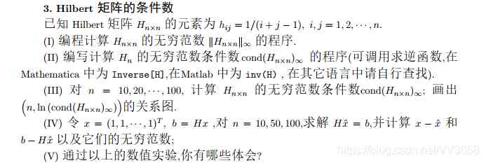
One 、 topic 3——Hilbert The condition number of a matrix

1. Title Description

** subject ：** You'll see .

2.python Realization

import numpy as np
import matplotlib.pyplot as plt
plt.rcParams['font.sans-serif'] = ['simhei']

n = int(input(' Please enter Hilbert The maximum dimension of a square matrix :' ))
def max_sum_rows(X):
    sum_row_list1 = []
    for i in range(len(X)):
        count = 0
        for j in range(len(X)):
            count += abs(X[i][j])
        sum_row_list1.append(count)
    return max(sum_row_list1)

inf_fanshu = []
Hilbert_cond = []
for i in range(1, n+1):
    X = 1./(np.arange(1, i+1) + np.arange(0, i)[:, np.newaxis])
    invX = np.linalg.inv(X)
    a1 = max_sum_rows(invX)
    a2 = max_sum_rows(X)
    inf_fanshu.append(a2)
    H_cond = a1 * a2
    Hilbert_cond.append(H_cond)

# Calculation 10,20……100 Infinite norm condition number of 
Hilbert_cond_test = []
for j in range(n):
    if (j+1)%10 == 0:
        Hilbert_cond_test.append(Hilbert_cond[j])
print(' Generating dimensions from 10,20……100 Of Hilbert The row norm condition number of a matrix ：\n', Hilbert_cond_test)

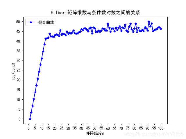
plt.title('Hilbert The relationship between matrix dimension and logarithm of condition number ')
plt.plot((list(range(1,n+1))), np.log(Hilbert_cond),c ='b', marker='*',label=' Fit the curve ')
plt.legend()
plt.xlabel(' Matrix dimensions n')
plt.xticks(np.arange(0, n+1, 5))
plt.yticks(np.arange(0, 55, 5))
plt.ylabel('log(cond)')
plt.show()

# solve Hilbert The solution of the equation and the corresponding infinite condition number 
r_A_A_acc_list = []
r_B_list = []
r_cond = []
r_B_cond = []
for i in range(1,n+1):
    A = np.ones((i,1))*1
    X = 1. / (np.arange(1, i + 1) + np.arange(0, i)[:, np.newaxis])
    B = X@A
    A_acc = np.linalg.inv(X)@B
    r_A_A_acc = A - A_acc
    r_B = B - X @ A_acc
    r_A_A_acc_list.append(r_A_A_acc)
    r_B_list.append(r_B)
    r_cond.append(abs(r_A_A_acc[:]).max()) #x-x_acc Infinite norm of 
    r_B_cond.append(abs(r_B[:]).max())#b-Hx_acc Infinite norm of 

print(' Dimension is 10,50,100 At the time of the x-x_acc The result of the calculation is ：\n', r_A_A_acc_list[9] ,r_A_A_acc_list[49] , r_A_A_acc_list[99])
print(' Dimension is 10,50,100 At the time of the b-Hx_acc The result of the calculation is ：\n',r_B_list[9], r_B_list[49], r_B_list[99])
print(' Dimension is 10,50,100 At the time of the x-x_acc The calculation result of infinite condition number of matrix ：\n', r_cond[9], r_cond[49], r_cond[99])
print(' Dimension is 10,50,100 At the time of the b-Hx_acc The calculation result of infinite condition number of matrix ：\n', r_B_cond[9], r_B_cond[49], r_B_cond[99])

3. Output results

Enter what you want to calculate Hilbert The maximum dimension of a square matrix is OK , Leave the rest to the program .

 Please enter Hilbert The maximum dimension of a square matrix :100
 Generating dimensions from 10,20……100 Of Hilbert The row norm condition number of a matrix ：
 [35356847610517.12, 6.008376652086652e+18, 8.396589803249062e+18, 9.491653209312077e+19, 1.7763569870536153e+20, 1.9301974218850052e+21, 3.9847310708042826e+19, 1.3450693870678838e+20, 5.444272740462528e+19, 1.3244131088115743e+20]

The output image here is as follows ：

Here is the output of the fourth question ：

 Dimension is 10,50,100 At the time of the x-x_acc The result of the calculation is ：
 [[-2.54168641e-04]
 [ 2.16242671e-03]
 [-5.54656982e-03]
 [ 5.08880615e-03]
 [ 9.15527344e-04]
 [-4.02832031e-03]
 [ 1.46484375e-03]
 [ 4.88281250e-04]
 [-1.22070312e-04]
 [-6.10351562e-05]] [[ 8.01768149e+02]
 [ 3.33788188e+04]
 [-1.59537467e+06]
 [ 1.98594595e+07]
 [-1.31128704e+08]
·················
 [-4.04700000e+03]
 [ 6.50000000e+01]
 [-2.25000000e+01]
 [ 3.30000000e+01]
 [-7.30000000e+01]] [[ 1.05255071e+04]
 [-1.31934071e+06]
 [ 4.56146227e+07]
 [-7.42843201e+08]
 [ 6.95696228e+09]
 [-4.13027099e+10]
 ················
 [-4.79000000e+02]
 [ 5.12100000e+03]
 [-1.91900000e+03]
 [ 1.77000000e+02]]
  Dimension is 10,50,100 At the time of the b-Hx_acc The result of the calculation is ：
 [[1.27400597e-05]
 [2.15601768e-05]
 [1.73587501e-05]
 [1.43429989e-05]
 [1.23056437e-05]
 [1.08422262e-05]
 [9.72981380e-06]
 [8.84754702e-06]
 [8.12566450e-06]
 [7.52108032e-06]] [[ 13.49201973]
 [  7.51301334]
 [ -4.25849823]
 [-14.49468816]
 [-21.55733783]
 [-26.46828937]
···············
 [-28.3616173 ]
 [-28.05340528]
 [-27.75051982]
 [-27.45291237]] [[-22.02594035]
 [-22.62163018]
 [-20.05848154]
 [-17.70284588]
 [-16.01064382]
 [-14.79343569]
···············
 [ -3.83066178]
 [ -3.79759674]
 [ -3.76500334]
 [ -3.73286444]
 [ -3.70119334]]

 Dimension is 10,50,100 At the time of the x-x_acc The calculation result of infinite condition number of matrix ：
 0.00554656982421875 7824513409.0 998313040247.0
 Dimension is 10,50,100 At the time of the b-Hx_acc The calculation result of infinite condition number of matrix ：
 2.1560176801216357e-05 38.404672581436365 22.62163018366762

Conclusion

Sharing is only for learning from each other , Discuss with each other , As the writing is wrong , Please forgive me a lot . Hope to learn from each other , Common progress , Welcome to leave a comment .