当前位置:网站首页>Word2vec (skip gram and cbow) - pytorch
Word2vec (skip gram and cbow) - pytorch
2022-07-06 22:48:00 【Gourd baby ah ah ah】
Hands on learning, deep learning notes
- Word vectors are vectors used to express the meaning of words , It can also be regarded as the feature vector of words . The technology of mapping words to real vectors is called word embedding .
One 、 Word embedding (Word2vec)
The unique heat vector cannot accurately express the similarity between different words ,word2vec The proposal of is to solve this problem , It maps each word to a fixed ⻓ The vector of degrees , These vectors can better express the similarity and analogy between different words .word2vec Contains two models :Skip-Gram and CBOW, Their training depends on conditional probability . Because it is data without labels , therefore Skip-Gram and CBOW Are self-monitoring models .
1.Skip-Gram
Skip-Gram: The head word predicts the surrounding words
Every word has Two d d d The vector representation of dimensions , Used to calculate conditional probability . The index in the dictionary is i i i Any word of , Use them separately v i ∈ R d \mathbf{v}_i\in\mathbb{R}^d vi∈Rd and u i ∈ R d \mathbf{u}_i\in\mathbb{R}^d ui∈Rd Represents two vectors when it is used as a head word and a context word . Given the central word w c w_c wc( The subscript indicates the index in the dictionary ), Generate any contextual words w o w_o wo The conditional probability of the vector dot product can be obtained by softmax Operation to model :
P ( w o ∣ w c ) = exp ( u o ⊤ v c ) ∑ i ∈ V exp ( u i ⊤ v c ) (1) P(w_o \mid w_c) = \frac{\text{exp}(\mathbf{u}_o^\top \mathbf{v}_c)}{ \sum_{i \in \mathcal{V}} \text{exp}(\mathbf{u}_i^\top \mathbf{v}_c)}\tag{1} P(wo∣wc)=∑i∈Vexp(ui⊤vc)exp(uo⊤vc)(1)
among , Thesaurus index set V = { 0 , 1 , … , ∣ V ∣ − 1 } \mathcal{V} = \{0, 1, \ldots, |\mathcal{V}|-1\} V={ 0,1,…,∣V∣−1}.
Given length is T T T The text sequence of , Among them, the time step t t t The word in place means w ( t ) w^{(t)} w(t). It is assumed that the context word is generated independently given any central word . For context windows m m m,Skip-Gram The likelihood function of is the probability of generating all context words given any central word :
∏ t = 1 T ∏ − m ≤ j ≤ m , j ≠ 0 P ( w ( t + j ) ∣ w ( t ) ) (2) \prod_{t=1}^{T} \prod_{-m \leq j \leq m,\ j \neq 0} P(w^{(t+j)} \mid w^{(t)})\tag{2} t=1∏T−m≤j≤m, j=0∏P(w(t+j)∣w(t))(2)
2.CBOW Model
CBOW: The surrounding words predict the central word
because CBOW There are multiple contextual words in , Therefore, when calculating the conditional probability, these context word vectors are averaged . For the index in the dictionary i i i Any word of , Use them separately v i ∈ R d \mathbf{v}_i\in\mathbb{R}^d vi∈Rd and u i ∈ R d \mathbf{u}_i\in\mathbb{R}^d ui∈Rd Represents two vectors used as context words and head words ( Symbols and Skip-Gram On the contrary ). Given the context word w o 1 , … , w o 2 m w_{o_1}, \ldots, w_{o_{2m}} wo1,…,wo2m( The index in the thesaurus is o 1 , … , o 2 m o_1, \ldots, o_{2m} o1,…,o2m) Generate any headword w c w_c wc The conditional probability of is :
P ( w c ∣ w o 1 , … , w o 2 m ) = exp ( 1 2 m u c ⊤ ( v o 1 + … , + v o 2 m ) ) ∑ i ∈ V exp ( 1 2 m u i ⊤ ( v o 1 + … , + v o 2 m ) ) (3) P(w_c \mid w_{o_1}, \ldots, w_{o_{2m}}) = \frac{\text{exp}\left(\frac{1}{2m}\mathbf{u}_c^\top (\mathbf{v}_{o_1} + \ldots, + \mathbf{v}_{o_{2m}}) \right)}{ \sum_{i \in \mathcal{V}} \text{exp}\left(\frac{1}{2m}\mathbf{u}_i^\top (\mathbf{v}_{o_1} + \ldots, + \mathbf{v}_{o_{2m}}) \right)}\tag{3} P(wc∣wo1,…,wo2m)=∑i∈Vexp(2m1ui⊤(vo1+…,+vo2m))exp(2m1uc⊤(vo1+…,+vo2m))(3)
Given length is T T T The text sequence of , Among them, the time step t t t The word in place means w ( t ) w^{(t)} w(t). For context windows m m m,CBOW The likelihood function of is the probability of generating all the central words given their context words :
∏ t = 1 T P ( w ( t ) ∣ w ( t − m ) , … , w ( t − 1 ) , w ( t + 1 ) , … , w ( t + m ) ) (4) \prod_{t=1}^{T} P(w^{(t)} \mid w^{(t-m)}, \ldots, w^{(t-1)}, w^{(t+1)}, \ldots, w^{(t+m)})\tag{4} t=1∏TP(w(t)∣w(t−m),…,w(t−1),w(t+1),…,w(t+m))(4)
Two 、 Negative sampling and layering softmax
Skip-Gram The main idea is to use softmax Operation to calculate based on the given central word w c w_c wc Generate upper and lower text w o w_o wo Conditional probability of . because softmax The nature of the operation , Context words can be word lists V \mathcal{V} V Any item in , The sum of items with the same size as the whole vocabulary . therefore , Skip-Gram Gradient calculation and CBOW All gradient calculations involve summation . But usually a dictionary has hundreds of thousands or millions of words , The computational cost of summing the gradient is huge !
In order to reduce the computational complexity , Let's say Skip-Gram As an example, learn two approximate calculation methods : Negative sampling and layered softmax.
1. Negative sampling
Given the central word w c w_c wc Context window for , Any context word w o w_o wo Events from this context window are considered to be probability modeled by :
P ( D = 1 ∣ w c , w o ) = σ ( u o ⊤ v c ) = exp ( u o ⊤ v c ) 1 + exp ( u o ⊤ v c ) = 1 1 + exp ( − u o ⊤ v c ) (5) P(D=1\mid w_c, w_o) = \sigma(\mathbf{u}_o^\top \mathbf{v}_c)\\= \frac{\exp(\mathbf{u}_o^\top \mathbf{v}_c)}{1+\exp(\mathbf{u}_o^\top \mathbf{v}_c)}\\= \frac{1}{1+\exp(-\mathbf{u}_o^\top \mathbf{v}_c)}\tag{5} P(D=1∣wc,wo)=σ(uo⊤vc)=1+exp(uo⊤vc)exp(uo⊤vc)=1+exp(−uo⊤vc)1(5)
Before negative sampling softmax( Many classification ), Now it is sigmoid( Two classification ).
Two classification , Multi classification can see the previous Logistic regression and multiple logistic regression This blog , The actual combat can be seen Logic returns to actual combat - Stock customer churn early warning model (Python Code ) This .
Maximize joint probability , Given length is T T T The text sequence of , With w ( t ) w^{(t)} w(t) Time step t t t The word , The context window is m m m, Formula for :
∏ t = 1 T ∏ − m ≤ j ≤ m , j ≠ 0 P ( D = 1 ∣ w ( t ) , w ( t + j ) ) (6) \prod_{t=1}^{T} \prod_{-m \leq j \leq m,\ j \neq 0} P(D=1\mid w^{(t)}, w^{(t+j)})\tag{6} t=1∏T−m≤j≤m, j=0∏P(D=1∣w(t),w(t+j))(6)
However , The formula 6 Consider only those events with positive samples . Only when all word vectors are equal to infinity , The joint probability is maximized to 1. Of course , Such a result is meaningless . In order to make the objective function more meaningful , Negative sampling adds negative samples sampled from a predefined distribution .
use S S S Context words w o w_o wo From the central word w c w_c wc Context window events . For this involves w o w_o wo Events , From predefined distribution P ( w ) P(w) P(w) In the sample K K K This is not from this context window Noise words . use N k N_k Nk Words indicating noise w k w_k wk( k = 1 , … , K k=1, \ldots, K k=1,…,K) Not from w c w_c wc Context window events . Suppose positive and negative cases S , N 1 , … , N K S, N_1, \ldots, N_K S,N1,…,NK These events are independent of each other . Negative sampling will be the original Skip-Gram The joint probability of ( The formula 2) rewrite , Change the conditional probability to the following formula :
P ( w ( t + j ) ∣ w ( t ) ) ≈ P ( D = 1 ∣ w ( t ) , w ( t + j ) ) ∏ k = 1 , w k ∼ P ( w ) K P ( D = 0 ∣ w ( t ) , w k ) P(w^{(t+j)} \mid w^{(t)})\approx\\ P(D=1\mid w^{(t)}, w^{(t+j)})\prod_{k=1,\ w_k \sim P(w)}^K P(D=0\mid w^{(t)}, w_k) P(w(t+j)∣w(t))≈P(D=1∣w(t),w(t+j))k=1, wk∼P(w)∏KP(D=0∣w(t),wk)
The loss function is negative log likelihood , Now the calculation cost of gradient is no longer related to the size of vocabulary , But with the number of noise words in negative sampling K K K( It's a super parameter , K K K The smaller the calculation cost, the lower ) of .
2. layered Softmax
layered Softmax Use a binary tree , Each leaf node of the tree represents a vocabulary V \mathcal{V} V One of the words in .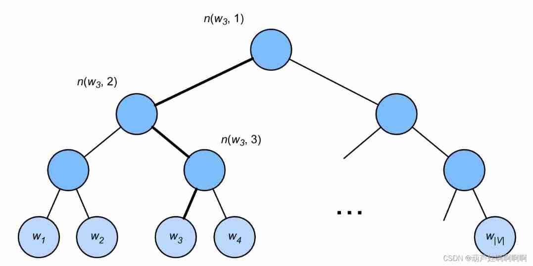
use L ( w ) L(w) L(w) Represents the word in the binary tree w w w The number of nodes on the path from the root node to the leaf node ( Including both ends ). set up n ( w , j ) n(w,j) n(w,j) For j t h j^\mathrm{th} jth node , The upper and lower text vectors are u n ( w , j ) \mathbf{u}_{n(w, j)} un(w,j).
for example , L ( w 3 ) = 4 L(w_3) = 4 L(w3)=4. layered softmax The conditional probability is approximated as
P ( w o ∣ w c ) ≈ ∏ j = 1 L ( w o ) − 1 σ ( [ [ n ( w o , j + 1 ) = leftChild ( n ( w o , j ) ) ] ] ⋅ u n ( w o , j ) ⊤ v c ) P(w_o \mid w_c) \approx \prod_{j=1}^{L(w_o)-1} \sigma\left( [\![ n(w_o, j+1) = \text{leftChild}(n(w_o, j)) ]\!] \cdot \mathbf{u}_{n(w_o, j)}^\top \mathbf{v}_c\right) P(wo∣wc)≈j=1∏L(wo)−1σ([[n(wo,j+1)=leftChild(n(wo,j))]]⋅un(wo,j)⊤vc)
among , leftChild ( n ) \text{leftChild}(n) leftChild(n) Is the node n n n The left child of : If x x x It's true , [ [ x ] ] = 1 [\![x]\!] = 1 [[x]]=1; otherwise [ [ x ] ] = − 1 [\![x]\!] = -1 [[x]]=−1.
To calculate the given word in the above figure w c w_c wc Generative word w 3 w_3 w3 Take the conditional probability of . This needs to be w c w_c wc The word of the vector v c \mathbf{v}_c vc And from root to w 3 w_3 w3 The path of ( The bold path in the figure ) Dot product between non leaf node vectors on , The path turns left 、 Traverse right and left :
P ( w 3 ∣ w c ) = σ ( u n ( w 3 , 1 ) ⊤ v c ) ⋅ σ ( − u n ( w 3 , 2 ) ⊤ v c ) ⋅ σ ( u n ( w 3 , 3 ) ⊤ v c ) P(w_3 \mid w_c) = \sigma(\mathbf{u}_{n(w_3, 1)}^\top \mathbf{v}_c) \cdot \sigma(-\mathbf{u}_{n(w_3, 2)}^\top \mathbf{v}_c) \cdot \sigma(\mathbf{u}_{n(w_3, 3)}^\top \mathbf{v}_c) P(w3∣wc)=σ(un(w3,1)⊤vc)⋅σ(−un(w3,2)⊤vc)⋅σ(un(w3,3)⊤vc)
from σ ( x ) + σ ( − x ) = 1 \sigma(x)+\sigma(-x) = 1 σ(x)+σ(−x)=1, It believes that based on arbitrary words w c w_c wc Generate a vocabulary V \mathcal{V} V The sum of conditional probabilities of all words in is 1: ∑ w ∈ V P ( w ∣ w c ) = 1. \sum_{w \in \mathcal{V}} P(w \mid w_c) = 1. ∑w∈VP(w∣wc)=1.
In a binary tree structure , L ( w o ) − 1 L(w_o)-1 L(wo)−1 About and O ( log 2 ∣ V ∣ ) \mathcal{O}(\text{log}_2|\mathcal{V}|) O(log2∣V∣) It's an order of magnitude . When the vocabulary size V \mathcal{V} V When a large , Compared with those without similar training , Use layering softmax The computational cost of each training step of is significantly reduced .
Summary
- Negative sampling constructs a loss function by considering independent events , These events involve both positive and negative cases . The calculation amount of training is linear with the number of noise words at each step .
- layered softmax Use the path from the root node to the leaf node in the binary tree to construct the loss function . The calculation cost of training depends on the logarithm of the size of the vocabulary .
3、 ... and 、 Data set for pre training word embedding
The dataset used here is Penn Tree Bank(PTB). The corpus is taken from “ Wall Street journal ” The article , Divided into training sets 、 Validation set and test set . In the original format , Each line of the text file represents a sentence separated by spaces . ad locum , We treat each word as a lexical element .
import math
import os
import random
import torch
from torch import nn
from d2l import torch as d2l
from torch.nn import functional as F

d2l.DATA_HUB['ptb'] = (d2l.DATA_URL + 'ptb.zip',
                       '319d85e578af0cdc590547f26231e4e31cdf1e42')


def read_ptb():
    """ take PTB The dataset is loaded into the list of text rows """
    data_dir = d2l.download_extract('ptb')
    # Read the training set.
    with open(os.path.join(data_dir, 'ptb.train.txt')) as f:
        raw_text = f.read()
    return [line.split() for line in raw_text.split('\n')]
- Building a vocabulary , Less than 10 The second word will be written by “<unk>” Lexical substitution .
sentences = read_ptb() # sentences Count : 42069
vocab = d2l.Vocab(sentences, min_freq=10) # vocab size: 6719
1. Down sampling
Text data usually has “the”、“a” and “in” And other high-frequency words , These words provide little useful information . Besides , A lot of ( high frequency ) Words will make the training speed very slow . therefore , When training words are embedded in the model , High frequency words can be down sampled . That is, every word in the dataset w i w_i wi Will be discarded with probability
P ( w i ) = max ( 1 − t f ( w i ) , 0 ) P(w_i) = \max\left(1 - \sqrt{\frac{t}{f(w_i)}}, 0\right) P(wi)=max(1−f(wi)t,0)
among , P ( w i ) P(w_i) P(wi) Refers to the probability of being discarded , f ( w i ) f(w_i) f(wi) Refer to words w i w_i wi Frequency of occurrence in the dataset , Constant t t t It's a super parameter. ( The following code is set to 1 0 − 4 10^{-4} 10−4). Only when f ( w i ) > t f(w_i) > t f(wi)>t when ,( high frequency ) word w i w_i wi Can be discarded , f ( w i ) f(w_i) f(wi) The higher the , The higher the probability of being discarded .
- Down sampling high-frequency words
def subsample(sentences, vocab):
    """ Down sampling high-frequency words """
    #  Exclude unknown lexical elements '<unk>'
    sentences = [[token for token in line if vocab[token] != vocab.unk]
                 for line in sentences]
    counter = d2l.count_corpus(sentences)
    num_tokens = sum(counter.values())

    #  If word elements are preserved during downsampling , Then return to True
    # counter[token]:token Frequency of ;num_tokens: The total token Number ( It doesn't contain <unk>)
    def keep(token):
        return(random.uniform(0, 1) <
               math.sqrt(1e-4 / counter[token] * num_tokens))

    return ([[token for token in line if keep(token)] for line in sentences],
            counter)

subsampled, counter = subsample(sentences, vocab)
- After down sampling , The number of samples of high-frequency words will be significantly reduced , The sampling number of low-frequency words will not change , Keep it all
def compare_counts(token):
    return (f'"{
      token}" The number of :'
            f' Before ={
      sum([l.count(token) for l in sentences])}, '
            f' after ={
      sum([l.count(token) for l in subsampled])}')
''' def compare_counts(token): return (f'"{token}" The number of :' f' Before ={counter[token]},' f' after ={d2l.count_corpus(subsampled)[token]}') '''
print(compare_counts('in'))
print(compare_counts('join'))
# "in" The number of : Before =18000,  after =1191
# "join" The number of : Before =45,  after =45
2. Extraction of head words and context words
The size of the context window is 1 To max_window_size The random value
def get_centers_and_contexts(corpus, max_window_size):
    """ return Skip-Gram The head word and context word of """
    centers, contexts = [], []
    for line in corpus:
        #  To form “ Central word - Context words ” Yes , Each sentence should have at least 2 Word
        if len(line) < 2:
            continue
        centers += line
        for i in range(len(line)):  #  In the middle of the context window i
            window_size = random.randint(1, max_window_size)
            indices = list(range(max(0, i - window_size),
                                 min(len(line), i + 1 + window_size)))
            #  Exclude the head word from the context word
            indices.remove(i)
            contexts.append([line[idx] for idx in indices])
    # centers: contain corpus All the words ,contexts: Context of all headwords
    return centers, contexts
3. Negative sampling
The noise words are sampled according to the predefined distribution , Sampling distribution through variables sampling_weights Pass on
class RandomGenerator:
    """ according to n Sample weights in {1,...,n} Randomly selected from """
    def __init__(self, sampling_weights):
        # Exclude
        self.population = list(range(1, len(sampling_weights) + 1))
        self.sampling_weights = sampling_weights
        self.candidates = []
        self.i = 0

    def draw(self):
        if self.i == len(self.candidates):
            #  cache k Random sampling results
            self.candidates = random.choices(
                self.population, self.sampling_weights, k=10000)
            self.i = 0
        self.i += 1
        return self.candidates[self.i - 1]
For a pair of head words and context words , Random sampling K K K individual ( In the experiment, there was no significant difference 5 individual ) Noise words . according to word2vec Suggestions in the paper , Put noise words w w w The sampling probability of P ( w ) P(w) P(w) Set to its relative frequency in the dictionary , Its power is 0.75.
def get_negatives(all_contexts, vocab, counter, K):
    """ Return the noise words in negative sampling """
    #  The index for 1、2、...( Indexes 0 Is an unknown tag excluded from the vocabulary )
    sampling_weights = [counter[vocab.to_tokens(i)]**0.75
                        for i in range(1, len(vocab))]
    all_negatives, generator = [], RandomGenerator(sampling_weights)
    for contexts in all_contexts:
        negatives = []
        while len(negatives) < len(contexts) * K:
            neg = generator.draw()
            #  Noise words cannot be context words
            if neg not in contexts:
                negatives.append(neg)
        all_negatives.append(negatives)
    return all_negatives
sentences = read_ptb()
vocab = d2l.Vocab(sentences, min_freq=10)
subsampled, counter = subsample(sentences, vocab)
#  After down sampling , Map lexical elements to their indexes in the corpus
corpus = [vocab[line] for line in subsampled]
all_centers, all_contexts = get_centers_and_contexts(corpus, 5)
all_negatives = get_negatives(all_contexts, vocab, counter, 5)
4. Load training instances in small batches
In small batches , i t h i^\mathrm{th} ith Samples include headwords and their n i n_i ni Context words and m i m_i mi A noise word . Because the size of the context window is different , n i + m i n_i+m_i ni+mi For different i i i Is different . therefore , For each sample , We are contexts_negatives Variables link their context words with noise words , And fill in zero , Until the connection length reaches max_len.
Mask variables masks In order to exclude filling in the calculation of loss . In order to distinguish positive and negative examples , Definition labels Variables separate context words from noise words . among labels Medium 1 Corresponding to contexts_negatives Positive examples of context words in ,0 Corresponding to negative example .
Input data Is a list with length equal to batch size , Each of these elements is composed of a central word center、 Its contextual words context And its noise words negative Sample of composition .
def batchify(data):
    """ Returns... With negative sampling Skip-Gram Small batch samples """
    max_len = max(len(c) + len(n) for _, c, n in data)
    centers, contexts_negatives, masks, labels = [], [], [], []
    for center, context, negative in data:
        cur_len = len(context) + len(negative)
        centers += [center]
        contexts_negatives += \
            [context + negative + [0] * (max_len - cur_len)]
        masks += [[1] * cur_len + [0] * (max_len - cur_len)]
        labels += [[1] * len(context) + [0] * (max_len - len(context))]
    return (torch.tensor(centers).reshape((-1, 1)), torch.tensor(
        contexts_negatives), torch.tensor(masks), torch.tensor(labels))
- Define function read PTB Data sets and returns data iterators and vocabularies
def load_data_ptb(batch_size, max_window_size, num_noise_words):
    """ download PTB Data sets , Then load it into memory """
    sentences = read_ptb()
    vocab = d2l.Vocab(sentences, min_freq=10)
    subsampled, counter = subsample(sentences, vocab)
    corpus = [vocab[line] for line in subsampled]
    all_centers, all_contexts = get_centers_and_contexts(corpus, max_window_size)
    all_negatives = get_negatives(all_contexts, vocab, counter, num_noise_words)

    class PTBDataset(torch.utils.data.Dataset):
        def __init__(self, centers, contexts, negatives):
            assert len(centers) == len(contexts) == len(negatives)
            self.centers = centers
            self.contexts = contexts
            self.negatives = negatives

        def __getitem__(self, index):
            return (self.centers[index], self.contexts[index],
                    self.negatives[index])

        def __len__(self):
            return len(self.centers)

    dataset = PTBDataset(all_centers, all_contexts, all_negatives)
    data_iter = torch.utils.data.DataLoader(dataset, batch_size,
                                    shuffle=True, collate_fn=batchify)
    return data_iter, vocab
- Print the first small batch of the data iterator
data_iter, vocab = load_data_ptb(512, 5, 5)
for batch in data_iter:
    for name, data in zip(names, batch):
        print(name, 'shape:', data.shape)
    break
centers shape: torch.Size([512, 1])
contexts_negatives shape: torch.Size([512, 60])
masks shape: torch.Size([512, 60])
labels shape: torch.Size([512, 60])
Four 、 Preliminary training word2vec
batch_size, max_window_size, num_noise_words = 512, 5, 5
data_iter, vocab = d2l.load_data_ptb(batch_size, max_window_size, num_noise_words)
1. Forward propagation
In forward propagation ,Skip-Gram The input of includes the headword index center( Batch size ,1) And context and noise word index contexts_and_negatives( Batch size ,max_len). These two variables are first converted from the lexical index into vectors through the embedding layer , Then multiply their batch matrix to return the shape ( Batch size ,1,max_len) Output . Each element in the output is the dot product of the central word vector and the context or noise word vector .
def skip_gram(center, contexts_and_negatives, embed_v, embed_u):
    v = embed_v(center)
    u = embed_u(contexts_and_negatives)
    pred = torch.bmm(v, u.permute(0, 2, 1))
    return pred
2. Loss function
class SigmoidBCELoss(nn.Module):
    """ Binary cross entropy loss with mask """
    def __init__(self):
        super().__init__()

    def forward(self, inputs, target, mask=None):
        out = F.binary_cross_entropy_with_logits(
            inputs, target, weight=mask, reduction="none")
        return out.mean(dim=1)

loss = SigmoidBCELoss()
- Initialize model parameters
embed_size = 100
net = nn.Sequential(nn.Embedding(num_embeddings=len(vocab),
                                 embedding_dim=embed_size),
                    nn.Embedding(num_embeddings=len(vocab),
                                 embedding_dim=embed_size))
3. Training
def train(net, data_iter, lr, num_epochs, device=d2l.try_gpu()):
def init_weights(m):
if type(m) == nn.Embedding:
nn.init.xavier_uniform_(m.weight)
net.apply(init_weights)
net = net.to(device)
optimizer = torch.optim.Adam(net.parameters(), lr=lr)
animator = d2l.Animator(xlabel='epoch', ylabel='loss', xlim=[1, num_epochs])
# Sum of normalized losses , Normalized loss number
metric = d2l.Accumulator(2)
for epoch in range(num_epochs):
timer, num_batches = d2l.Timer(), len(data_iter)
for i, batch in enumerate(data_iter):
optimizer.zero_grad()
center, context_negative, mask, label = [data.to(device) for data in batch]
pred = skip_gram(center, context_negative, net[0], net[1])
l = (loss(pred.reshape(label.shape).float(), label.float(), mask)
/ mask.sum(axis=1) * mask.shape[1])
l.sum().backward()
optimizer.step()
metric.add(l.sum(), l.numel())
if (i + 1) % (num_batches // 5) == 0 or i == num_batches - 1:
animator.add(epoch + (i + 1) / num_batches,
(metric[0] / metric[1],))
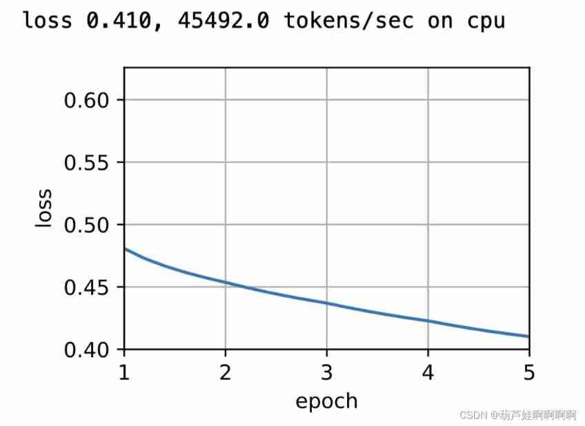
print(f'loss {
metric[0] / metric[1]:.3f}, '
f'{
metric[1] / timer.stop():.1f} tokens/sec on {
str(device)}')
lr, num_epochs = 0.002, 5
train(net, data_iter, lr, num_epochs)
4. Word embedding
Training word2vec After the model , You can use the cosine similarity of the word vector in the trained model to find the word with the most similar semantics to the input word from the vocabulary .
def get_similar_tokens(query_token, k, embed):
    W = embed.weight.data
    x = W[vocab[query_token]]
    #  Calculate cosine similarity . increase 1e-9 To obtain numerical stability
    cos = torch.mv(W, x) / torch.sqrt(torch.sum(W * W, dim=1) *
                                      torch.sum(x * x) + 1e-9)
    # torch.topk(cos, k=k+1)[1]  Return to the top of the similarity in descending order k+1 Corresponding indexes
    topk = torch.topk(cos, k=k+1)[1].cpu().numpy().astype('int32')
    for i in topk[1:]:  #  Delete the input word
        print(f'cosine sim={
      float(cos[i]):.3f}: {
      vocab.to_tokens(i)}')

get_similar_tokens('chip', 3, net[0])
边栏推荐
- TypeScript获取函数参数类型
- QT signal and slot
- Cloud native technology container knowledge points
- 存币生息理财dapp系统开发案例演示
- config:invalid signature 解决办法和问题排查详解
- void关键字
- That's why you can't understand recursion
- 「小程序容器技术」,是噱头还是新风口?
- [IELTS speaking] Anna's oral learning record part1
- The ceiling of MySQL tutorial. Collect it and take your time
猜你喜欢
Sword finger offer question brushing record 1

UE4 blueprint learning chapter (IV) -- process control forloop and whileloop
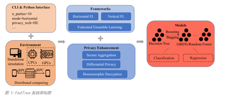
Designed for decision tree, the National University of Singapore and Tsinghua University jointly proposed a fast and safe federal learning system
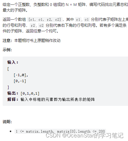
leetcode:面试题 17.24. 子矩阵最大累加和(待研究)
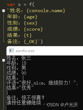
Aardio - 通过变量名将变量值整合到一串文本中
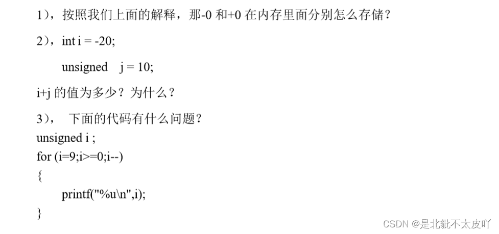
Signed and unsigned keywords
![[leetcode] 19. Delete the penultimate node of the linked list](/img/ab/25cb6d6538ad02d78f7d64b2a2df3f.png)
[leetcode] 19. Delete the penultimate node of the linked list

config:invalid signature 解决办法和问题排查详解

Cocoscreator+typescripts write an object pool by themselves
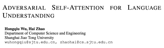
ICLR 2022 | pre training language model based on anti self attention mechanism
随机推荐
AdaViT——自适应选择计算结构的动态网络
poj 1094 Sorting It All Out (拓扑排序)
雅思口语的具体步骤和时间安排是什么样的?
Windows auzre background operation interface of Microsoft's cloud computing products
Aardio - 利用customPlus库+plus构造一个多按钮组件
General implementation and encapsulation of go diversified timing tasks
【Unity】升级版·Excel数据解析,自动创建对应C#类,自动创建ScriptableObject生成类,自动序列化Asset文件
Const keyword
Motion capture for snake motion analysis and snake robot development
cuda 探索
UVa 11732 – strcmp() Anyone?
Classification, function and usage of MySQL constraints
2014阿里巴巴web前实习生项目分析(1)
【踩坑合辑】Attempting to deserialize object on CUDA device+buff/cache占用过高+pad_sequence
How to confirm the storage mode of the current system by program?
Signed and unsigned keywords
void关键字
HDU 5077 NAND (violent tabulation)
Chapter 19 using work queue manager (2)
BasicVSR_PlusPlus-master测试视频、图片