当前位置:网站首页>Opencv learning notes 9 -- background modeling + optical flow estimation
Opencv learning notes 9 -- background modeling + optical flow estimation
2022-07-06 07:32:00 【Cloudy_ to_ sunny】
opencv Study notes 9 -- Background modeling + Optical flow estimation
Background modeling
Frame difference method
Because the target in the scene is moving , The image of the target has different positions in different image frames . This kind of algorithm performs differential operation on two consecutive images in time , The pixels corresponding to different frames are subtracted , Judge the absolute value of gray difference , When the absolute value exceeds a certain threshold , It can be judged as a moving target , So as to realize the detection function of the target .

The frame difference method is very simple , But it will introduce noise and cavity problems
Gaussian mixture model
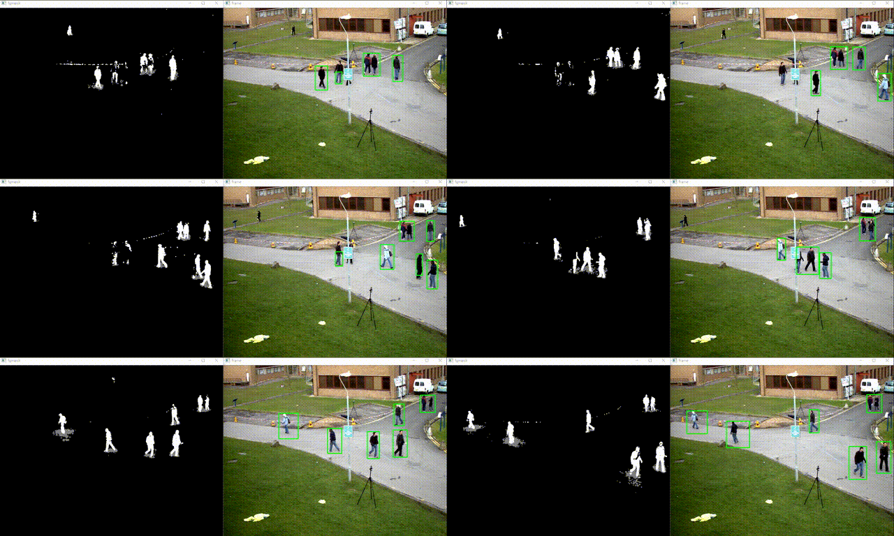
Before foreground detection , First train the background , A Gaussian mixture model is used to simulate each background in the image , The number of Gaussian mixtures per background can be adaptive . Then in the test phase , Update the new pixel GMM matching , If the pixel value can match one of the Gauss , It is considered to be the background , Otherwise, it is considered a prospect . Because of the whole process GMM The model is constantly updating and learning , Therefore, it has certain robustness to dynamic background . Finally, through the foreground detection of a dynamic background with branch swing , Good results have been achieved .
In the video, the change of pixels should conform to Gaussian distribution

The actual distribution of the background should be a mixture of multiple Gaussian distributions , Each Gaussian model can also be weighted

Gaussian mixture model learning method
1. First initialize each Gaussian model matrix parameter .
2. Take the video T Frame data image is used to train Gaussian mixture model . After you get the first pixel, use it as the first Gaussian distribution .
3. When the pixel value comes later , Compared with the previous Gaussian mean , If the difference between the value of the pixel and its model mean is within 3 Within the variance of times , It belongs to this distribution , And update its parameters .
4. If the next pixel does not meet the current Gaussian distribution , Use it to create a new Gaussian distribution .
Gaussian mixture model test method
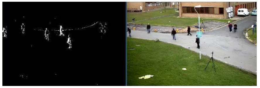
In the test phase , Compare the value of the new pixel with each mean in the Gaussian mixture model , If the difference is 2 Times the variance between words , It is considered to be the background , Otherwise, it is considered a prospect . Assign the foreground to 255, The background is assigned to 0. In this way, a foreground binary map is formed .
import numpy as np
import cv2

# Classic test video
cap = cv2.VideoCapture('test.avi')
# Morphological operations need to use , Used to remove noise
kernel = cv2.getStructuringElement(cv2.MORPH_ELLIPSE,(3,3))
# Create Gaussian mixture model for background modeling
fgbg = cv2.createBackgroundSubtractorMOG2()

while(True):
    ret, frame = cap.read()
    fgmask = fgbg.apply(frame)
    # Morphological operation to remove noise
    fgmask = cv2.morphologyEx(fgmask, cv2.MORPH_OPEN, kernel)
    # Find the outline in the video
    im, contours, hierarchy = cv2.findContours(fgmask, cv2.RETR_EXTERNAL, cv2.CHAIN_APPROX_SIMPLE)

    for c in contours:
        # Calculate the perimeter of each profile
        perimeter = cv2.arcLength(c,True)
        if perimeter > 188:
            # Find a straight rectangle ( Won't rotate )
            x,y,w,h = cv2.boundingRect(c)
            # Draw this rectangle
            cv2.rectangle(frame,(x,y),(x+w,y+h),(0,255,0),2)

    cv2.imshow('frame',frame)
    cv2.imshow('fgmask', fgmask)
    k = cv2.waitKey(150) & 0xff
    if k == 27:
        break

cap.release()
cv2.destroyAllWindows()
Optical flow estimation
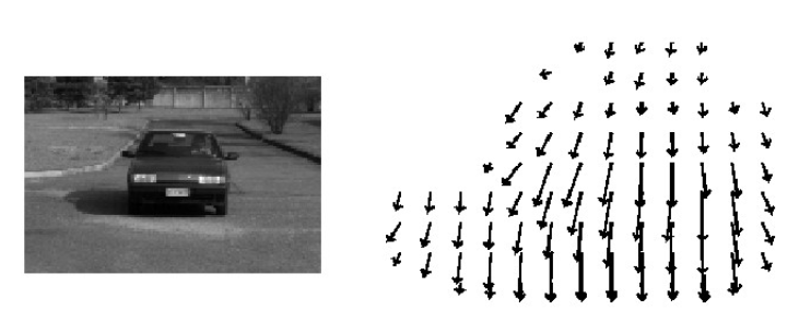
Optical flow is the result of the pixel motion of a space moving object on the observation imaging plane “ Instantaneous speed ”, According to the velocity vector characteristics of each pixel , The image can be dynamically analyzed , Target tracking, for example .
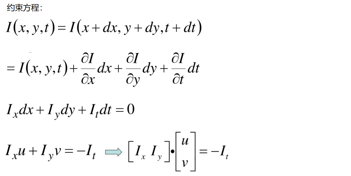
Brightness is constant : The same point changes over time , Its brightness will not change .
Small movement : The change over time will not cause a drastic change in position , Only in the case of small motion can the gray change caused by the change of unit position between the front and back frames be used to approximate the partial derivative of gray to position .
Spatial consistency : Adjacent points on a scene projected onto the image are also adjacent points , And the velocity of adjacent points is the same . Because there is only one constraint on the basic equation of optical flow method , And demand x,y Speed in direction , There are two unknown variables . So we need to stand together n Solve multiple equations .

Lucas-Kanade Algorithm
How to solve the equations ? It seems that one pixel is not enough , What other characteristics are there in the process of object movement ?( Corner reversible , So feature points use corners )
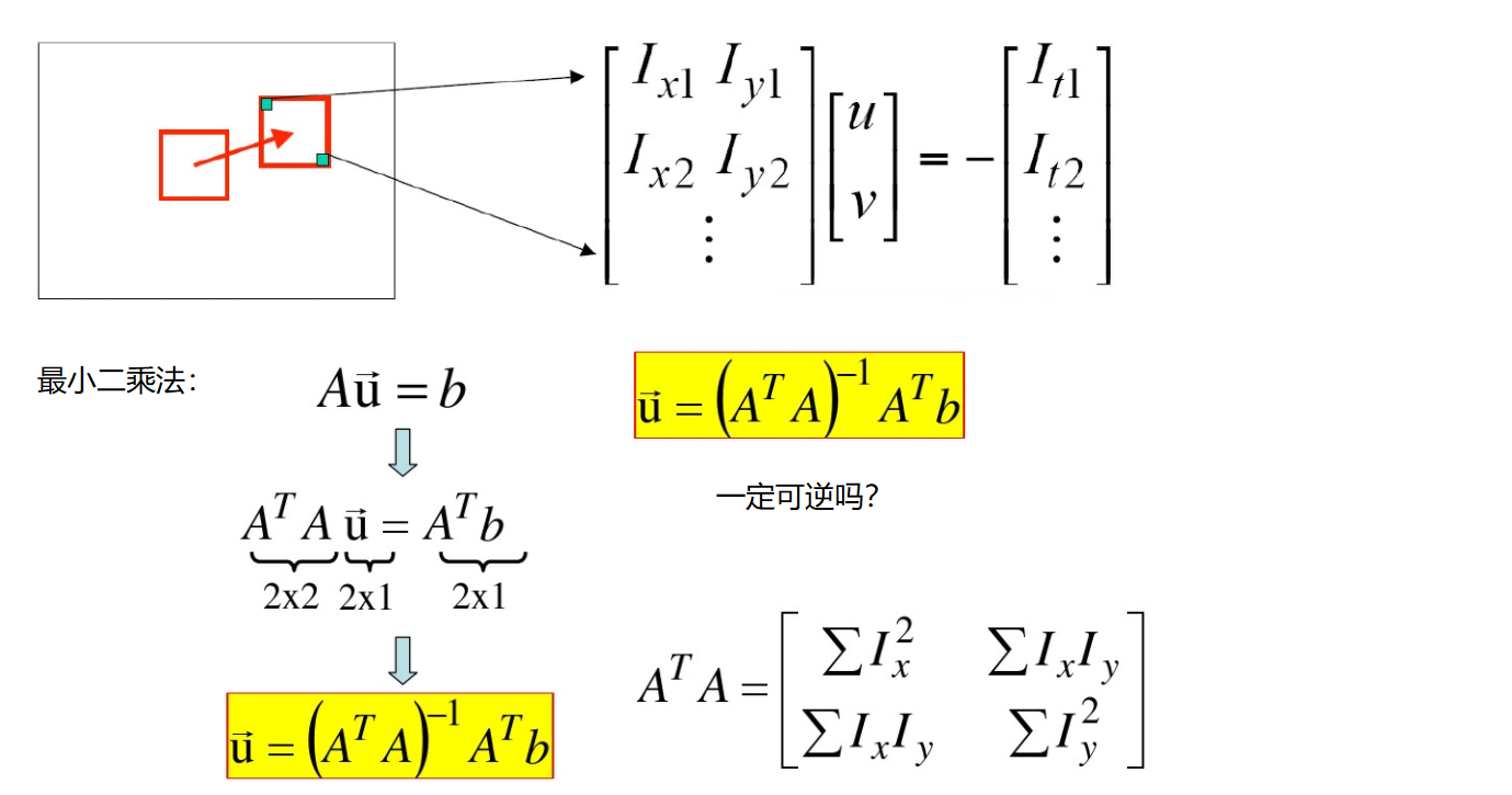
cv2.calcOpticalFlowPyrLK():
Parameters :
prevImage Previous frame image
nextImage The current frame image
prevPts Feature point vector to be tracked
winSize The size of the search window
maxLevel The largest number of pyramid layers
return :
nextPts Output tracking feature point vector
status Whether the feature points are found , The status found is 1, The status of not found is 0
import numpy as np
import cv2

cap = cv2.VideoCapture('test.avi')

#  Parameters required for corner detection
feature_params = dict( maxCorners = 100,
                       qualityLevel = 0.3,
                       minDistance = 7)

# lucas kanade Parameters
lk_params = dict( winSize  = (15,15),
                  maxLevel = 2)

#  Random color bar
color = np.random.randint(0,255,(100,3))

#  Get the first image
ret, old_frame = cap.read()
old_gray = cv2.cvtColor(old_frame, cv2.COLOR_BGR2GRAY)
#  Return all detected feature points , You need to enter an image , Maximum number of corners ( efficiency ), Quality factor ( The larger the eigenvalue, the better , To screen )
#  The distance is equivalent to that there is a stronger angle in this interval than this corner , I don't want this weak one
p0 = cv2.goodFeaturesToTrack(old_gray, mask = None, **feature_params)

#  Create a mask
mask = np.zeros_like(old_frame)

while(True):
    ret,frame = cap.read()
    frame_gray = cv2.cvtColor(frame, cv2.COLOR_BGR2GRAY)

    #  It is necessary to input the previous frame, the current image and the corner detected in the previous frame
    p1, st, err = cv2.calcOpticalFlowPyrLK(old_gray, frame_gray, p0, None, **lk_params)

    # st=1 Express
    good_new = p1[st==1]
    good_old = p0[st==1]

    #  Drawing tracks
    for i,(new,old) in enumerate(zip(good_new,good_old)):
        a,b = new.ravel()
        c,d = old.ravel()
        mask = cv2.line(mask, (a,b),(c,d), color[i].tolist(), 2)
        frame = cv2.circle(frame,(a,b),5,color[i].tolist(),-1)
    img = cv2.add(frame,mask)

    cv2.imshow('frame',img)
    k = cv2.waitKey(150) & 0xff
    if k == 27:
        break

    #  to update
    old_gray = frame_gray.copy()
    p0 = good_new.reshape(-1,1,2)

cv2.destroyAllWindows()
cap.release()
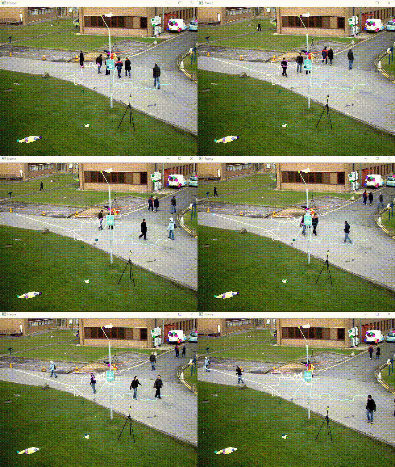
Reference resources
边栏推荐
- The differences and advantages and disadvantages between cookies, seeion and token
- Is the super browser a fingerprint browser? How to choose a good super browser?
- Go learning -- implementing generics based on reflection and empty interfaces
- jmeter性能测试步骤实战教程
- C - Inheritance - hidden method
- 杰理之BLE【篇】
- [MySQL learning notes 30] lock (non tutorial)
- Wonderful use of TS type gymnastics string
- Jerry's ad series MIDI function description [chapter]
- The ECU of 21 Audi q5l 45tfsi brushes is upgraded to master special adjustment, and the horsepower is safely and stably increased to 305 horsepower
猜你喜欢
杰理之BLE【篇】
Basics of reptile - Scratch reptile

How to delete all the words before or after a symbol in word

Crawling exercise: Notice of crawling Henan Agricultural University
Relevant introduction of clip image
杰理之BLE【篇】
杰理之如若需要大包发送,需要手机端修改 MTU【篇】
Significance and measures of encryption protection for intelligent terminal equipment

Go learning -- implementing generics based on reflection and empty interfaces
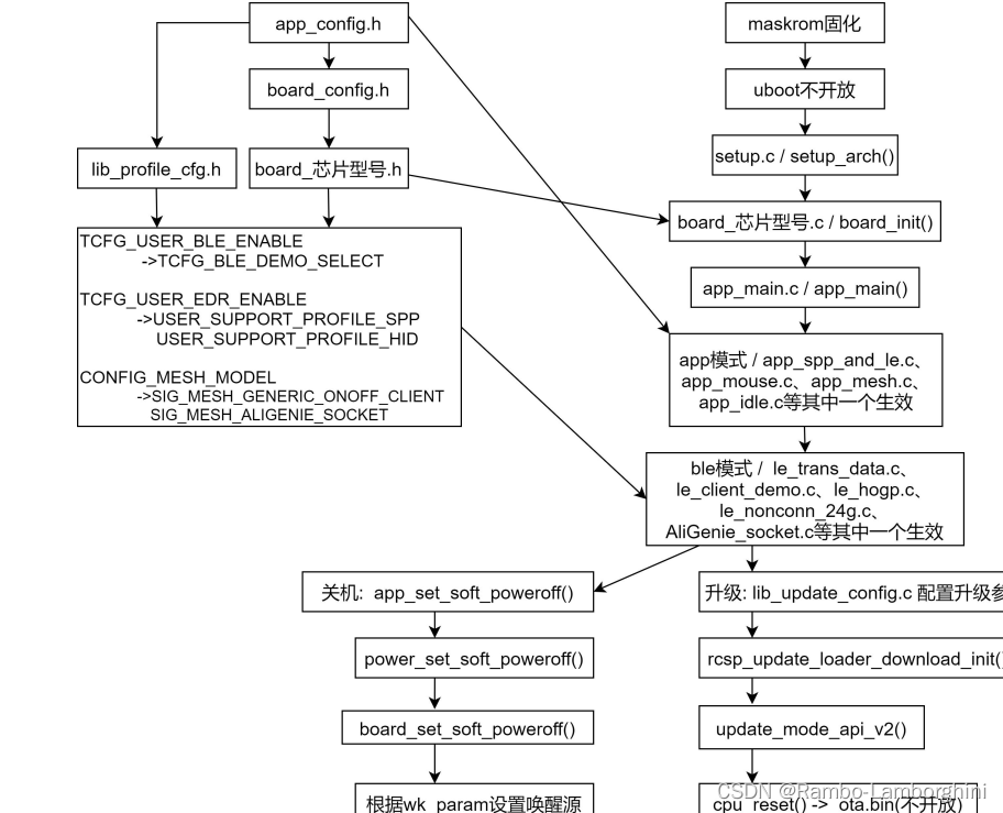
杰理之BLE【篇】
随机推荐
word设置目录
【线上问题处理】因代码造成mysql表死锁的问题,如何杀掉对应的进程
【mysql学习笔记30】锁(非教程)
QT color is converted to string and uint
Word setting directory
How can word delete English only and keep Chinese or delete Chinese and keep English
数字经济时代,如何保障安全?
Mise en œuvre du langage leecode - C - 15. Somme des trois chiffres - - - - - idées à améliorer
【mysql学习笔记29】触发器
Memory error during variable parameter overload
Go learning --- use reflection to judge whether the value is valid
OpenJudge NOI 2.1 1661:Bomb Game
The difference between TS Gymnastics (cross operation) and interface inheritance
Introduction to the basics of network security
杰理之普通透传测试---做数传搭配 APP 通信【篇】
学go之路(二)基本类型及变量、常量
C intercept string
杰理之BLE【篇】
杰理之开发板上电开机,就可以手机打开 NRF 的 APP【篇】
[CF Gym101196-I] Waif Until Dark 网络最大流