吴恩达机器学习课后习题——线性回归

单变量线性回归

import numpy as np
import pandas as pd
import matplotlib.pyplot as plt

path = "ex1data1.txt"
data = pd.read_csv(path, header=None, names=['Population', 'Profit'])
# pandas.read_csv默认情况下会把数据内容的第一行默认为字段名标题，header=None指明读取的原始文件数据没有列索引
data.head() # 方法用于返回数据帧或序列的前n行(默认值为5)。返回类型：DataFrame，可理解为一个表格，或者说矩阵
# DataFrame本质上是二维矩阵，跟常规二维矩阵的差别在于前者额外指定了每一行和每一列的名称。

	Population	Profit
0	6.1101	17.5920
1	5.5277	9.1302
2	8.5186	13.6620
3	7.0032	11.8540
4	5.8598	6.8233

data.describe()
# describe() 函数可以查看数据的基本情况，
# 包括：count 非空值数、mean 平均值、std 标准差、max 最大值、min 最小值、（25%、50%、75%）分位数等。

	Population	Profit
count	97.000000	97.000000
mean	8.159800	5.839135
std	3.869884	5.510262
min	5.026900	-2.680700
25%	5.707700	1.986900
50%	6.589400	4.562300
75%	8.578100	7.046700
max	22.203000	24.147000

# 画出图形
data.plot(kind='scatter',x='Population',y='Profit',figsize=(12,8))
# scatter表示散点图，figsize表示图片大小，单位：英寸
plt.show()

​

​

使用梯度下降来最小化代价函数,
创建一个以参数θ为特征函数的代价函数
$$J\left(\theta \right)=\frac{1}{2m}\sum _{i=1}^m{\left(h_{\theta }\left(x^{(i)}\right)-y^{(i)}\right)}^2$$
其中：
$$h_{\theta }\left(x\right)={\theta }^{T}X={\theta }_0{x}_0+{\theta }_1{x}_1+{\theta }_2{x}_2+...+{\theta }_n{x}_n$$

def computeCost(X,y,theta): # 输入X是列向量，y也是列向量，theta是行向量
    inner = np.power(((X*theta.T)-y),2) # x*θ的转置就是假设函数 power函数计算numpy数组中每个数值的指定幂次
    return np.sum(inner/(2*len(X))) # 将数组/矩阵中的元素全部加起来 len(X)矩阵行数

data.insert(0,'Ones',1)  
# 插入一列为1是为了更好的向量化，需要在训练集中添加一列x_0，以便我们可以使用向量化的解决方案来计算代价和梯度，见视频p18

# 变量的初始化
cols = data.shape[1] # shape[0]是行数 shape[1]是列数
X = data.iloc[:,0:cols-1] # 数据集 行全要 列从0到cols-1(不包括) 左闭右开
y = data.iloc[:,cols-1:cols] # 目标值
X.head()

	Ones	Population
0	1	6.1101
1	1	5.5277
2	1	8.5186
3	1	7.0032
4	1	5.8598

获取的数据类型是DataFrame类型，所以需要进行类型转换。同时还需要初始化theta,即theta所有元素都设置为0

X = np.matrix(X.values)
y = np.matrix(y.values)
theta = np.matrix(np.array([0,0]))

维度

X.shape, theta.shape, y.shape

((97, 2), (1, 2), (97, 1))

computeCost(X,y,theta) #计算代价函数

32.072733877455676

batch gradient decent（批量梯度下降）

$${\theta }_j:={\theta }_j-\alpha \frac{\partial }{\partial {\theta }_j}J\left(\theta \right)$$
梯度下降

def gradientDescent(X,y,theta,alpha,iters): # iters是迭代次数 alpha是学习率 即步长
    temp_theta = np.matrix(np.zeros(theta.shape)) # 零值矩阵 暂存theta
    parameters = int(theta.ravel().shape[1]) # ravel计算需要求解的参数个数 功能将多维数组降至一维 这里值为2
    cost = np.zeros(iters) #构建iters个0的数组
    #迭代：
    for i in range(iters):
        difference = (X*theta.T) - y # 差值
        for j in range(parameters):
            term = np.multiply(difference,X[:,j])    #乘以x_i X[:,j]表示所有行 j列，简言之就是抽出第j列 
             # 注意这里就不是矩阵乘法了 这里是求导后要求乘的 multiply是两个相同大小矩阵对应位置的数直接相乘
            temp_theta[0,j] = theta[0,j] - (alpha/len(X))*np.sum(term) # 更新theta_j
        
        theta = temp_theta # 更新全部theta值
        cost[i] = computeCost(X,y,theta) # 更新代价值
    
    return theta,cost

初始化一些附加变量 - 学习速率α和要执行的迭代次数。

alpha = 0.01
iters = 1000

获取theta值，代价最小值

g,cost = gradientDescent(X,y,theta,alpha,iters)
g

matrix([[-3.24140214,  1.1272942 ]])

cost[-1] # 获取数组的最后一个值

4.515955503078913

最后，用我们拟合过的theta值计算训练模型的代价函数

computeCost(X, y, g)

4.515955503078913

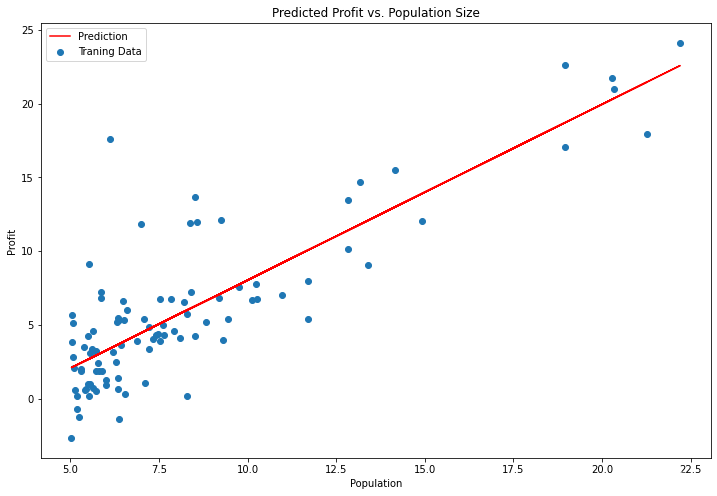
绘制线性模型以及数据，直观地看出它的拟合

x = np.linspace(data.Population.min(), data.Population.max(), 100) # 生成指定范围内指定个数的一维数组
f = g[0, 0] + (g[0, 1] * x) # x1=1 g[0, 0]表示theta_0 g[0, 1]表示theta_1

fig, ax = plt.subplots(figsize=(12,8)) # plt.subplot()函数用于直接指定划分方式和位置进行绘图。
# fig代表绘图窗口(Figure)；ax代表这个绘图窗口上的坐标系(axis)，一般会继续对ax进行操作。

# 设置横纵坐标的函数，并设置颜色为红色，在图标上标上'Prediction'标签 横坐标x 纵坐标f
ax.plot(x, f, 'r', label='Prediction') 
# 定义散点图的横纵坐标，并给出散点图点的'Traning Data'标签名
ax.scatter(data.Population, data.Profit, label='Traning Data') 
ax.legend(loc=2)  # 2表示在左上角


ax.set_xlabel('Population')
ax.set_ylabel('Profit')
ax.set_title('Predicted Profit vs. Population Size')
plt.show()

​

​

由于梯度方程式函数也在每个训练迭代中输出一个代价的向量，所以我们也可以绘制。 注意，代价总是降低

fig, ax = plt.subplots(figsize=(12,8))
ax.plot(np.arange(iters), cost, 'r')
ax.set_xlabel('Iterations')
ax.set_ylabel('Cost')
ax.set_title('Error vs. Training Epoch')
plt.show()

​

​

多变量的线性回归

该练习包括一个房屋价格数据集，其中包含两个变量（房屋大小、卧室数量）和目标（房子价格）。

path =  'ex1data2.txt'
data2 = pd.read_csv(path, header=None, names=['Size', 'Bedrooms', 'Price'])
data2.head()

	Size	Bedrooms	Price
0	2104	3	399900
1	1600	3	329900
2	2400	3	369000
3	1416	2	232000
4	3000	4	539900

data2.describe()

	Size	Bedrooms	Price
count	47.000000	47.000000	47.000000
mean	2000.680851	3.170213	340412.659574
std	794.702354	0.760982	125039.899586
min	852.000000	1.000000	169900.000000
25%	1432.000000	3.000000	249900.000000
50%	1888.000000	3.000000	299900.000000
75%	2269.000000	4.000000	384450.000000
max	4478.000000	5.000000	699900.000000

房屋大小约为卧室数量的1000倍。当特征相差几个数量级时，首先执行特征缩放（均值归一化）可以使梯度下降更快地收敛。

data2 = (data2 - data2.mean()) / data2.std() # 解决的方法是尝试将所有特征尺度都尽量缩放到 -1 ~ 1
data2.head()

	Size	Bedrooms	Price
0	0.130010	-0.223675	0.475747
1	-0.504190	-0.223675	-0.084074
2	0.502476	-0.223675	0.228626
3	-0.735723	-1.537767	-0.867025
4	1.257476	1.090417	1.595389

data2.insert(0, 'Ones', 1) 
cols = data2.shape[1]
X2 = data2.iloc[:,0:cols-1]
y2 = data2.iloc[:,cols-1:cols]

X2 = np.matrix(X2.values)
y2 = np.matrix(y2.values)
theta2 = np.matrix(np.array([0,0,0]))

g2, cost2 = gradientDescent(X2, y2, theta2, alpha, iters)
computeCost(X2, y2, g2) # 计算代价

0.1307033696077189

代价函数收敛图

fig, ax = plt.subplots(figsize=(12,8))
ax.plot(np.arange(iters), cost2, 'r')
ax.set_xlabel('Iterations')
ax.set_ylabel('Cost')
ax.set_title('Error vs. Training Epoch')
plt.show()

​

​

使用sklearn线性回归函数简化过程

from sklearn import linear_model
model = linear_model.LinearRegression()  #基于最小二乘法的线性回归。
model.fit(X, y)

x = np.array(X[:, 1].A1)
f = model.predict(X).flatten()

fig, ax = plt.subplots(figsize=(12,8))
ax.plot(x, f, 'r', label='Prediction')
ax.scatter(data.Population, data.Profit, label='Traning Data')
ax.legend(loc=2)
ax.set_xlabel('Population')
ax.set_ylabel('Profit')
ax.set_title('Predicted Profit vs. Population Size')
plt.show()

normal equation（正规方程）

思路

正规方程是通过求解下面的方程来找出使得代价函数最小的参数的：$\frac{\partial }{\partial {\theta }_j}J\left({\theta }_j\right)=0$ 。
假设我们的训练集特征矩阵为 X（包含了$x_0=1$）并且我们的训练集结果为向量 y，则利用正规方程解出向量 $\theta ={\left(X^{T}X\right)}^{-1}{X}^{T}y$ 。
上标T代表矩阵转置，上标-1 代表矩阵的逆。设矩阵$A=X^{T}X$，则：${\left(X^{T}X\right)}^{-1}=A^{-1}$

梯度下降与正规方程的比较：

梯度下降：需要选择学习率α，需要多次迭代，当特征数量n大时也能较好适用，适用于各种类型的模型
正规方程：不需要选择学习率α，一次计算得出，需要计算${\left(X^{T}X\right)}^{-1}$，如果特征数量n较大则运算代价大，因为矩阵逆的计算时间复杂度为$O(n3)$，通常来说当$n$小于10000 时还是可以接受的，只适用于线性模型，不适合逻辑回归模型等其他模型

# 正规方程函数
def normalEqn(X, y):
    theta = np.linalg.inv(X.[email protected])@X.[email protected]#[email protected]等价于X.T.dot(X) np.linalg.inv()：矩阵求逆
    return theta

final_theta2=normalEqn(X, y)
final_theta2  # 梯度matrix([[-3.24140214, 1.1272942 ]])

matrix([[-3.89578088],
        [ 1.19303364]])