当前位置:网站首页>[CV] Wu Enda machine learning course notes | Chapter 12
[CV] Wu Enda machine learning course notes | Chapter 12
2022-07-02 21:24:00 【Fannnnf】
If there is no special explanation in this series of articles , The text explains the picture above the text
machine learning | Coursera
Wu Enda machine learning series _bilibili
Catalog
12 Support vector machine (SVM)
12-1 Optimization objectives

- The coordinate system on the left of the above figure is y = 1 y=1 y=1 Image of time valence function , Support vector machine draws a pink curve , Name it C o s t 1 ( z ) Cost_1(z) Cost1(z), Subscript refers to y y y The value of is 1 1 1
- alike , The right coordinate system is y = 0 y=0 y=0 Image of time valence function , Support vector machine draws a pink curve , Name it C o s t 0 ( z ) Cost_0(z) Cost0(z), Subscript refers to y y y The value of is 0 0 0
In logical regression , The cost function is :
J ( θ ) = − 1 m [ ∑ i = 1 m y ( i ) l o g ( h θ ( x ( i ) ) ) + ( 1 − y ( i ) ) l o g ( 1 − h θ ( x ( i ) ) ) ] + λ 2 m ∑ j = 1 n θ j 2 J(θ)=-\frac{1}{m}\left[\sum_{i=1}^my^{(i)}log(h_θ(x^{(i)}))+(1-y^{(i)})log(1-h_θ(x^{(i)}))\right]+\frac{λ}{2m}\sum_{j=1}^{n}θ_j^2 J(θ)=−m1[i=1∑my(i)log(hθ(x(i)))+(1−y(i))log(1−hθ(x(i)))]+2mλj=1∑nθj2
Support vector machine , First put the minus sign in the above formula into the sum , And then put 1 m \frac{1}{m} m1 Get rid of ( 1 m \frac{1}{m} m1 It's a constant , Although removing it will change the value of the cost function , But the same minimum value can still be obtained θ \theta θ), The resulting cost function is :
J ( θ ) = ∑ i = 1 m [ y ( i ) ( − l o g ( h θ ( x ( i ) ) ) ) + ( 1 − y ( i ) ) ( − l o g ( 1 − h θ ( x ( i ) ) ) ) ] + λ 2 ∑ j = 1 n θ j 2 J(θ)=\sum_{i=1}^m\left[y^{(i)}\left (-log(h_θ(x^{(i)}))\right )+(1-y^{(i)})\left(-log(1-h_θ(x^{(i)}))\right)\right]+\frac{λ}{2}\sum_{j=1}^{n}θ_j^2 J(θ)=i=1∑m[y(i)(−log(hθ(x(i))))+(1−y(i))(−log(1−hθ(x(i))))]+2λj=1∑nθj2
Put... In the above formula ( − l o g ( h θ ( x ( i ) ) ) ) \left (-log(h_θ(x^{(i)}))\right ) (−log(hθ(x(i)))) Replace with C o s t 1 ( θ T x ( i ) ) Cost_1(\theta^Tx^{(i)}) Cost1(θTx(i)), hold ( − l o g ( 1 − h θ ( x ( i ) ) ) ) \left(-log(1-h_θ(x^{(i)}))\right) (−log(1−hθ(x(i)))) Replace with C o s t 0 ( θ T x ( i ) ) Cost_0(\theta^Tx^{(i)}) Cost0(θTx(i)), Get the cost function :
J ( θ ) = ∑ i = 1 m [ y ( i ) C o s t 1 ( θ T x ( i ) ) + ( 1 − y ( i ) ) C o s t 0 ( θ T x ( i ) ) ] + λ 2 ∑ j = 1 n θ j 2 J(θ)=\sum_{i=1}^m\left[y^{(i)}Cost_1(\theta^Tx^{(i)})+(1-y^{(i)})Cost_0(\theta^Tx^{(i)})\right]+\frac{λ}{2}\sum_{j=1}^{n}θ_j^2 J(θ)=i=1∑m[y(i)Cost1(θTx(i))+(1−y(i))Cost0(θTx(i))]+2λj=1∑nθj2
In support vector machines , No longer use regularization parameters λ \lambda λ, Use parameters instead C C C, The cost function of the changed support vector machine is :
J ( θ ) = C ∑ i = 1 m [ y ( i ) C o s t 1 ( θ T x ( i ) ) + ( 1 − y ( i ) ) C o s t 0 ( θ T x ( i ) ) ] + 1 2 ∑ j = 1 n θ j 2 J(θ)=C\sum_{i=1}^m\left[y^{(i)}Cost_1(\theta^Tx^{(i)})+(1-y^{(i)})Cost_0(\theta^Tx^{(i)})\right]+\frac{1}{2}\sum_{j=1}^{n}θ_j^2 J(θ)=Ci=1∑m[y(i)Cost1(θTx(i))+(1−y(i))Cost0(θTx(i))]+21j=1∑nθj2
- Support vector machines do not predict y = 1 / 0 y=1/0 y=1/0 Probability , If θ T x ( i ) ≥ 0 \theta^Tx^{(i)}\ge0 θTx(i)≥0, Suppose the function output 1, On the contrary, output 0
12-2 Understanding of large spacing
Support vector machine is also called large space classifier 
Change the judgment boundary in support vector machine , Give Way θ T x ( i ) ≥ 1 \theta^Tx^{(i)}\ge1 θTx(i)≥1 When the output 1, θ T x ( i ) ≤ − 1 \theta^Tx^{(i)}\le-1 θTx(i)≤−1 When the output 0, In this way, there is a safe gap between the two results 
Using a general logistic regression algorithm may generate pink and green lines in the above figure to segment two types of samples , And use support vector chance to generate black lines in the figure , The area between the two blue lines in the figure is called the spacing , Support vector machines try to separate the two samples with the greatest spacing , It can be seen that , Support vector machine can have better robustness 
Pictured above , Let's assume that there is no negative sample on the left , Use a big C C C The black line in the above figure can be generated , But if there is a negative sample on the left , because C C C It's big , Support vector machine is used to ensure the maximum distance between two kinds of samples , The pink line in the above figure will be generated , But if C C C It's not that big , Then even if there is a negative sample on the left , Black lines will still be generated
- C C C It's equivalent to the previous 1 λ \frac{1}{\lambda} λ1, Although the two are really different , But the effect is similar
12-3 Mathematical principle of support vector machine
12-4 Kernel function I
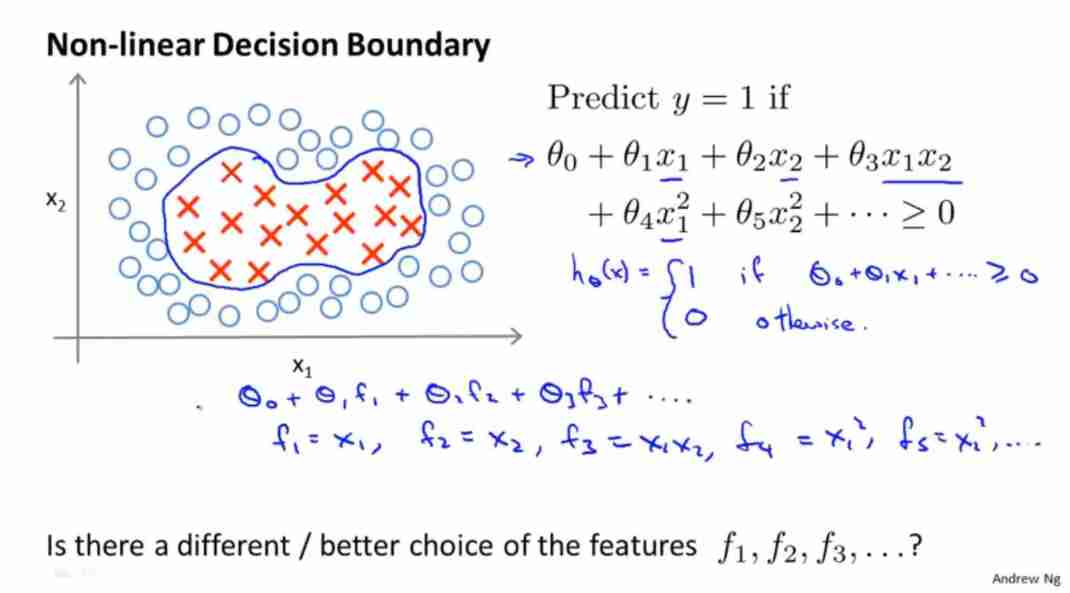
The sample shown in the figure , If we assume that the function ≥ 0 \ge0 ≥0, Just predict y = 1 y=1 y=1, Other predictions y = 0 y=0 y=0,
In the hypothetical function in the figure above , set up f 1 = x 1 , f 2 = x 2 , f 3 = x 1 x 2 , f 4 = x 1 2 , . . . f_1=x_1,f_2=x_2,f_3=x_1x_2,f_4=x_1^2,... f1=x1,f2=x2,f3=x1x2,f4=x12,...
Suppose the function becomes h θ ( x ) = θ 0 + θ 1 f 1 + θ 2 f 2 + . . . h_\theta(x)=\theta_0+\theta_1 f_1+\theta_2 f_2+... hθ(x)=θ0+θ1f1+θ2f2+...
The above method has nothing to do with the following method , Independent of kernel function
However , In addition to combining the original features , Is there a better way to construct 𝑓1, 𝑓2, 𝑓3? We can use kernel function to calculate new features .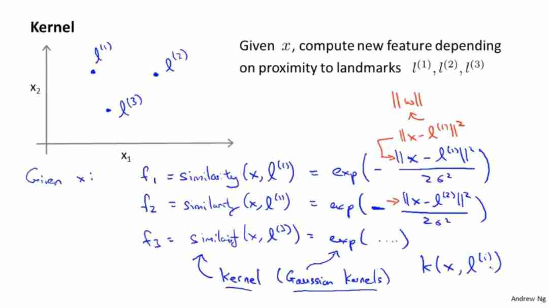
Take... In the coordinate system 3 Sample marking matrix l ( 1 ) 、 l ( 2 ) 、 l ( 3 ) l^{(1)}、l^{(2)}、l^{(3)} l(1)、l(2)、l(3)
x x x Is a given training example , Suppose there are two eigenvalues , that x = [ x 1 , x 2 ] x=[x_1,x_2] x=[x1,x2]
Make
f 1 = s i m i l a r i t y ( x , l ( 1 ) ) = e x p ( − ∥ x − l ( 1 ) ∥ 2 2 σ 2 ) f_1=similarity\left(x,l^{(1)}\right)=exp\left(-\frac{\Vert x-l^{(1)} \Vert ^2}{2\sigma^2}\right) f1=similarity(x,l(1))=exp(−2σ2∥x−l(1)∥2)
f 2 = s i m i l a r i t y ( x , l ( 2 ) ) = e x p ( − ∥ x − l ( 2 ) ∥ 2 2 σ 2 ) f_2=similarity\left(x,l^{(2)}\right)=exp\left(-\frac{\Vert x-l^{(2)} \Vert^2 }{2\sigma^2}\right) f2=similarity(x,l(2))=exp(−2σ2∥x−l(2)∥2)
f 3 = . . . . . . f_3=...... f3=......
. . . . . . ...... ......
- s i m i l a r i t y ( x , l ( i ) ) similarity\left(x,l^{(i)}\right) similarity(x,l(i)) It is called similarity measure function / Kernel function
- s i m i l a r i t y ( x , l ( i ) ) similarity\left(x,l^{(i)}\right) similarity(x,l(i)) It can also be written as k ( x , l ( i ) ) k\left(x,l^{(i)}\right) k(x,l(i))
- e x p ( x ) exp(x) exp(x) Express e x e^x ex, It is called Gaussian kernel function
- σ 2 \sigma^2 σ2 Is the parameter of Gaussian kernel function
The kernel function can be reduced to :
f 1 = s i m i l a r i t y ( x , l ( 1 ) ) = e x p ( − ∥ x − l ( 1 ) ∥ 2 2 σ 2 ) = e x p ( − ∑ j = 1 n ( x j − l j ( 1 ) ) 2 2 σ 2 ) f_1=similarity\left(x,l^{(1)}\right)=exp\left(-\frac{\Vert x-l^{(1)} \Vert ^2}{2\sigma^2}\right)=exp\left(-\frac{\sum_{j=1}^n(x_j-l_j^{(1)} )^2}{2\sigma^2}\right) f1=similarity(x,l(1))=exp(−2σ2∥x−l(1)∥2)=exp(−2σ2∑j=1n(xj−lj(1))2)
If x x x Very close to the mark l ( 1 ) l^{(1)} l(1), that f 1 ≈ e x p ( − 0 2 2 σ 2 ) ≈ 1 f_1\approx exp(-\frac{0^2}{2\sigma^2})\approx1 f1≈exp(−2σ202)≈1
If x x x Stay away from the mark l ( 1 ) l^{(1)} l(1), that f 1 ≈ e x p ( − ( l a r g e n u m b e r ) 2 2 σ 2 ) ≈ 0 f_1\approx exp(-\frac{(large\ number)^2}{2\sigma^2})\approx0 f1≈exp(−2σ2(large number)2)≈0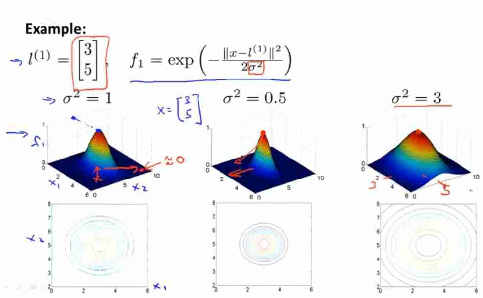
Upper figure , If σ 2 \sigma^2 σ2 Bigger , that f i f_i fi The descent speed of will slow down ( The slope decreases )
Pictured above , Take a little x x x, It has been calculated by support vector machine θ 0 、 θ 1 、 . . . \theta_0、\theta_1、... θ0、θ1、... The value of is shown in the figure above , Then we can calculate according to the kernel function f 0 、 f 1 、 . . . f_0、f_1、... f0、f1、... The value of is shown in the figure above , take θ \theta θ and f f f The value of is substituted into the assumed function to get 0.5 ≥ 0 0.5\ge0 0.5≥0, So predict y = 1 y=1 y=1
Pictured above , Take another point x x x, hypothesis : Finally get close l ( 1 ) and l ( 2 ) l^{(1)} and l^{(2)} l(1) and l(2) The point of will be predicted as 1, And away l ( 1 ) and l ( 2 ) l^{(1)} and l^{(2)} l(1) and l(2) The point of will be predicted as 0, Finally, you can fit a red curve as shown in the figure , The prediction in the curve is 1, The prediction outside the curve is 0
12-5 Kernel function II
How to choose landmarks ?
We usually choose the number of landmarks according to the number of training sets , That is, if there is 𝑚 An example , Then we choose
take 𝑚 Landmarks , And make :𝑙(1) = 𝑥(1), 𝑙(2) = 𝑥(2), . . . . . , 𝑙(𝑚) = 𝑥(𝑚). The advantage of doing so is : Now we
The new features are based on the distance between the original features and all other features in the training set , namely :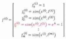

from
f 1 ( i ) = s i m i l a r i t y ( x ( i ) , l ( 1 ) ) f_1^{(i)}=similarity\left(x^{(i)},l^{(1)}\right) f1(i)=similarity(x(i),l(1))
f 2 ( i ) = s i m i l a r i t y ( x ( i ) , l ( 2 ) ) f_2^{(i)}=similarity\left(x^{(i)},l^{(2)}\right) f2(i)=similarity(x(i),l(2))
. . . ... ...
f m ( i ) = s i m i l a r i t y ( x ( i ) , l ( m ) ) f_m^{(i)}=similarity\left(x^{(i)},l^{(m)}\right) fm(i)=similarity(x(i),l(m))
take f f f Write as eigenvector form to get
f ( i ) = [ f 0 ( i ) = 1 f 1 ( i ) f 2 ( i ) . . . f m ( i ) ] f^{(i)}= \begin{bmatrix} f_0^{(i)}=1\\ f_1^{(i)}\\ f_2^{(i)}\\ ...\\ f_m^{(i)} \end{bmatrix} f(i)=⎣⎢⎢⎢⎢⎢⎡f0(i)=1f1(i)f2(i)...fm(i)⎦⎥⎥⎥⎥⎥⎤
f ( i ) f^{(i)} f(i) It's a m + 1 m+1 m+1 D matrix , Because except for m m m Out of samples , A bias term is also added f 0 ( i ) = 1 f_0^{(i)}=1 f0(i)=1
matrix f ( i ) f^{(i)} f(i) The meaning is ( The first i i i All the features in the samples ) And ( from 1 To m All the features in each sample ) Perform kernel operation , altogether m The operation results are arranged in the matrix , And add the 0 One of the f 0 ( i ) = 1 f_0^{(i)}=1 f0(i)=1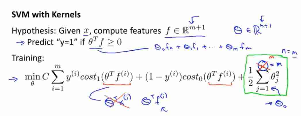
use f ( i ) f^{(i)} f(i) Replacement tape x x x term , The cost function obtained is :
C ∑ i = 1 m [ y ( i ) C o s t 1 ( θ T f ( i ) ) + ( 1 − y ( i ) ) C o s t 0 ( θ T f ( i ) ) ] + 1 2 ∑ j = 1 n = m θ j 2 C\sum_{i=1}^m\left[y^{(i)}Cost_1(\theta^Tf^{(i)})+(1-y^{(i)})Cost_0(\theta^Tf^{(i)})\right]+\frac{1}{2}\sum_{j=1}^{n=m}θ_j^2 Ci=1∑m[y(i)Cost1(θTf(i))+(1−y(i))Cost0(θTf(i))]+21j=1∑n=mθj2
- On the regularization term n = m n=m n=m The explanation of : θ ( i ) \theta_{(i)} θ(i) Is corresponding to matrix f ( i ) f^{(i)} f(i) The weight of , Because there are i = 1 , 2 , . . . , m i=1,2,...,m i=1,2,...,m common m individual f ( i ) f^{(i)} f(i) Corresponding m individual θ \theta θ, So let's assume that there are m term , That is to say m individual θ \theta θ, And the weight has been specified before θ \theta θ Number of n To express , So there's n = m n=m n=m Note that this has been ignored θ 0 \theta_0 θ0, Don't regularize it
The regularization term is in concrete implementation , The summation part can be written as ∑ j = 1 n = m θ j 2 = θ T θ \sum_{j=1}^{n=m}θ_j^2=\theta^T\theta ∑j=1n=mθj2=θTθ, And use θ T M θ \theta^TM\theta θTMθ Instead of θ T θ \theta^T\theta θTθ, matrix M M M It's a matrix that varies according to the kernel function we choose , This can improve the computational efficiency , The modified cost function is :
C ∑ i = 1 m [ y ( i ) C o s t 1 ( θ T f ( i ) ) + ( 1 − y ( i ) ) C o s t 0 ( θ T f ( i ) ) ] + 1 2 θ T M θ C\sum_{i=1}^m\left[y^{(i)}Cost_1(\theta^Tf^{(i)})+(1-y^{(i)})Cost_0(\theta^Tf^{(i)})\right]+\frac{1}{2}\theta^TM\theta Ci=1∑m[y(i)Cost1(θTf(i))+(1−y(i))Cost0(θTf(i))]+21θTMθ
Theoretically speaking , We can also use kernel functions in logistic regression , But it uses 𝑀 The method to simplify the calculation is not suitable for logistic regression , So computing is going to be very time consuming .
Here it is , We do not introduce a method to minimize the cost function of support vector machines , You can use existing packages ( Such as
liblinear,libsvm etc. ). Before we use these packages to minimize our cost function , We usually need to write a core
function , And if we use Gaussian kernel functions , So it is necessary to scale features before using them .
in addition , Support vector machines can also use no kernel function , Not using kernel function is also called linear kernel function (linear kernel),
When we don't use very complex functions , Or when we have a lot of features in our training set and very few examples , Can pick
Use this support vector machine without kernel function .
Here are two parameters for SVM 𝐶 and 𝜎 Influence :
𝐶 = 1/𝜆
𝐶 large , amount to 𝜆 smaller , May cause over fitting , High variance ;
𝐶 More hours , amount to 𝜆 more , May cause low fit , High deviation ;
𝜎 large , May lead to low variance , High deviation ;
𝜎 More hours , May cause low deviation , High variance .
come from https://www.cnblogs.com/sl0309/p/10499278.html

The above figure shows the influence of two parameters on the result
12-6 Using support vector machines (SVM)

- Use SVM Software library to calculate θ \theta θ Value
- We need to choose C Value
- We need to choose kernel function
- Linear kernel function : Do not select kernel function , Use linear fitting directly , It can be found in the number of features n It's big , And the number of samples m Use in very small cases
- Gaussian kernel : It can be found in the number of samples m It's big , Number of features n Use in very small cases , It can fit the nonlinear boundary
When using nonlinear kernel function , The eigenvalues need to be normalized
The kernel function needs to satisfy the mersel theorem Mercer’s theorem

边栏推荐
- [shutter] statefulwidget component (floatingactionbutton component | refreshindicator component)
- Volvo's first MPV is exposed! Comfortable and safe, equipped with 2.0T plug-in mixing system, it is worth first-class
- Welfare, let me introduce you to someone
- 想问问,现在开户有优惠吗?在线开户是安全么?
- rwctf2022_ QLaaS
- ctf-HCTF-Final-Misc200
- I want to ask you, where is a better place to open an account in Dongguan? Is it safe to open a mobile account?
- China Indonesia advanced wound care market trend report, technological innovation and market forecast
- What is the difference between programming in real work and that in school?
- Accounting regulations and professional ethics [19]
猜你喜欢
![[question brushing diary] classic questions of dynamic planning](/img/31/fcd8230f809d6178f11e7095c1ef94.jpg)
[question brushing diary] classic questions of dynamic planning
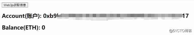
Web3js method to obtain account information and balance

Redis sentinel cluster working principle and architecture deployment # yyds dry goods inventory #

ROS learning (10): ROS records multiple topic scripts
![[error record] the command line creates an error pub get failed (server unavailable) -- attempting retry 1 in 1 second](/img/6e/c82ff02a249b5d275a4589120a197a.jpg)
[error record] the command line creates an error pub get failed (server unavailable) -- attempting retry 1 in 1 second

Detailed upgrade process of AWS eks
Huawei Hongmeng watch achieves fireworks display effect on New Year's Eve
![[shutter] shutter layout component (Introduction to layout component | row component | column component | sizedbox component | clipoval component)](/img/45/735431f59a84e9554225a72a551ab8.jpg)
[shutter] shutter layout component (Introduction to layout component | row component | column component | sizedbox component | clipoval component)

Research Report on ranking analysis and investment strategic planning of RFID market competitiveness of China's industrial manufacturing 2022-2028 Edition
![[cloud native topic -50]:kubesphere cloud Governance - operation - step by step deployment of microservice based business applications - database middleware MySQL microservice deployment process](/img/e6/1dc747de045166f09ecdce1c5a34b1.jpg)
[cloud native topic -50]:kubesphere cloud Governance - operation - step by step deployment of microservice based business applications - database middleware MySQL microservice deployment process
随机推荐
Research Report on the overall scale, major manufacturers, major regions, products and application segmentation of signal distributors in the global market in 2022
MySQL learning notes (Advanced)
Market trend report, technical dynamic innovation and market forecast of China's low gloss instrument
Don't you want to have a face-to-face communication with cloud native and open source experts? (including benefits
What is online account opening? Is it safe to open an account online now?
Interpretation of some papers published by Tencent multimedia laboratory in 2021
想请教一下,究竟有哪些劵商推荐?手机开户是安全么?
ctf-HCTF-Final-Misc200
6 pyspark Library
JDBC | Chapter 3: SQL precompile and anti injection crud operation
Research Report on ranking analysis and investment strategic planning of RFID market competitiveness of China's industrial manufacturing 2022-2028 Edition
[12] the water of the waves is clear, which can wash my tassel. The water of the waves is muddy, which can wash my feet
I would like to ask what securities dealers recommend? Is it safe to open a mobile account?
Construction and maintenance of business website [5]
Structured text language XML
China Indonesia advanced wound care market trend report, technological innovation and market forecast
rwctf2022_ QLaaS
Construction and maintenance of business websites [10]
qwb2018_ core kernel_ rop
Welfare | Pu Aries | liv heart co branded Plush surrounding new products are on the market!