怎么利用Tensorflow2进行猫狗分类识别

这篇文章主要讲解了“怎么利用Tensorflow2进行猫狗分类识别”，文中的讲解内容简单清晰，易于学习与理解，下面请大家跟着小编的思路慢慢深入，一起来研究和学习“怎么利用Tensorflow2进行猫狗分类识别”吧！

数据集获取

使用tf.keras.utils.get_file()能够从指定的URL当中直接获取数据集，我们在已知网站当中获取到猫狗分类所需图片，为压缩包格式，将其命名为cats_and_dogs_filtered.zip，为该操作设置一个变量path，该变量指向的便是该数据集下载之后存储的路径。

import tensorflow as tfpath=tf.keras.utils.get_file('cats_and_dogs_filtered.zip',origin='https://storage.googleapis.com/mledu-datasets/cats_and_dogs_filtered.zip')print(path)#会输出其路径，和当前notebook文件路径相同

文件解压

使用第三方库zipfile进行文件的解压，下列代码将其解压到了指定的文件夹当中。

import zipfilelocal_zip = pathzip_ref = zipfile.ZipFile(local_zip, 'r')zip_ref.extractall('C:\\Users\\lenovo\\.keras\\datasets')zip_ref.close()

文件夹当中又有两个文件夹，分别用于训练以及验证神经网络模型，每个文件夹当中又包含着两个文件，代表着不同类别的猫与狗的图片所处位置路径。

我们在一个神经网络模型的构建当中，需要训练集（train data）与验证集（validation data）。通俗而言，这里的训练集就是告诉模型猫与狗的外表。而验证集可以检查模型的好坏，评估模型的效果。

将文件分为训练集与验证集

使用os库找到猫狗数据的文件夹的路径，将其根据文件夹划分为数据集。

import osbase_dir = 'C:/Users/lenovo/.keras/datasets/cats_and_dogs_filtered'train_dir = os.path.join(base_dir, 'train')validation_dir = os.path.join(base_dir, 'validation')train_cats_dir = os.path.join(train_dir, 'cats')train_dogs_dir = os.path.join(train_dir, 'dogs')validation_cats_dir = os.path.join(validation_dir, 'cats')validation_dogs_dir = os.path.join(validation_dir, 'dogs')

下面来看一看train文件夹当中的cats文件夹和dogs文件夹当中的文件数据。

train_cat_fnames = os.listdir( train_cats_dir )train_dog_fnames = os.listdir( train_dogs_dir )print(train_cat_fnames[:10])print(train_dog_fnames[:10])

['cat.0.jpg', 'cat.1.jpg', 'cat.10.jpg', 'cat.100.jpg', 'cat.101.jpg', 'cat.102.jpg', 'cat.103.jpg', 'cat.104.jpg', 'cat.105.jpg', 'cat.106.jpg']['dog.0.jpg', 'dog.1.jpg', 'dog.10.jpg', 'dog.100.jpg', 'dog.101.jpg', 'dog.102.jpg', 'dog.103.jpg', 'dog.104.jpg', 'dog.105.jpg', 'dog.106.jpg']

同时查看文件当中包含图片数据数量的大小。

print('total training cat images :', len(os.listdir(train_cats_dir)))print('total training dog images :', len(os.listdir(train_dogs_dir)))print('total validation cat images :', len(os.listdir(validation_cats_dir)))print('total validation dog images :', len(os.listdir(validation_dogs_dir)))

total training cat images : 1000total training dog images : 1000total validation cat images : 500total validation dog images : 500

我们了解到对于猫和狗的数据集，我们都有1000张图片用于训练模型，500张图片用于验证模型效果。

绘图查看

下面对猫狗分类数据集图片进行输出，直观地观察不同图片的异同。

#设置画布大小以及子图个数%matplotlib inlineimport matplotlib.image as mpimgimport matplotlib.pyplot as pltnrows = 4ncols = 4pic_index = 0

绘制八只猫与八只狗图片，观看数据集中图片有哪些特征。

fig = plt.gcf()fig.set_size_inches(ncols*4, nrows*4)pic_index+=8next_cat_pix = [os.path.join(train_cats_dir, fname)                 for fname in train_cat_fnames[ pic_index-8:pic_index]                ]next_dog_pix = [os.path.join(train_dogs_dir, fname)                 for fname in train_dog_fnames[ pic_index-8:pic_index]               ]for i, img_path in enumerate(next_cat_pix+next_dog_pix):  sp = plt.subplot(nrows, ncols, i + 1)  sp.axis('Off')  img = mpimg.imread(img_path)  plt.imshow(img)plt.show()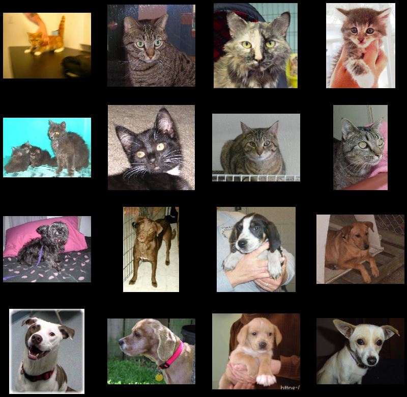

通过观察输出图片我们发现图片形状比例各不相同。与简单的手写数字集识别不同的是，手写数字集都是统一的28*28大小的灰度图片，而猫狗数据集是长宽各不同的彩色图片。

模型建立

神经网络模型

model = tf.keras.models.Sequential([    tf.keras.layers.Conv2D(16, (3,3), activation='relu', input_shape=(150, 150, 3)),    tf.keras.layers.MaxPooling2D(2,2),    tf.keras.layers.Conv2D(32, (3,3), activation='relu'),    tf.keras.layers.MaxPooling2D(2,2),     tf.keras.layers.Conv2D(64, (3,3), activation='relu'),     tf.keras.layers.MaxPooling2D(2,2),    tf.keras.layers.Flatten(),     tf.keras.layers.Dense(512, activation='relu'),     tf.keras.layers.Dense(1, activation='sigmoid')  ])

我们考虑将图片全部转化为150*150形状的图片，然后添加一系列的卷积层以及池化层，最后展平再进入DNN.

model.summary()#观察神经网络的参数

输出结果：

Model: "sequential"
_________________________________________________________________
Layer (type)                 Output Shape              Param #   
=================================================================
conv2d (Conv2D)              (None, 148, 148, 16)      448       
_________________________________________________________________
max_pooling2d (MaxPooling2D) (None, 74, 74, 16)        0         
_________________________________________________________________
conv2d_1 (Conv2D)            (None, 72, 72, 32)        4640      
_________________________________________________________________
max_pooling2d_1 (MaxPooling2 (None, 36, 36, 32)        0         
_________________________________________________________________
conv2d_2 (Conv2D)            (None, 34, 34, 64)        18496     
_________________________________________________________________
max_pooling2d_2 (MaxPooling2 (None, 17, 17, 64)        0         
_________________________________________________________________
flatten (Flatten)            (None, 18496)             0         
_________________________________________________________________
dense (Dense)                (None, 512)               9470464   
_________________________________________________________________
dense_1 (Dense)              (None, 1)                 513       
=================================================================
Total params: 9,494,561
Trainable params: 9,494,561
Non-trainable params: 0
_________________________________________________________________

Outshape显示了图片在神经网络中的尺寸变化情况，可以看到在连续的神经网络层当中，卷积层将图片尺寸不断缩小，而池化层一直让图片的尺寸减半。

模型编译

接下来我们将进行模型的编译。 我们将使用二值交叉熵binary_crossentropy损失训练我们的模型，因为这是一个二元分类问题，我们的最后一层的激活函数设置为sigmoid，我们将使用学习率为0.001的rmsprop优化器。在训练期间，我们将要监控分类的准确性。

在这种情况下，使用 RMSprop 优化算法比随机梯度下降 (SGD) 更可取，因为 RMSprop 为我们自动调整学习率。 （其他优化器例如Adam和Adagrad，也会在训练期间自动调整学习率，在这里也同样适用。）

from tensorflow.keras.optimizers import RMSpropmodel.compile(optimizer=RMSprop(lr=0.001),              loss='binary_crossentropy',              metrics = ['acc'])

数据预处理

让我们设置数据生成器，它将读取我们源文件夹中的图片，将它们转换为张量，并将它们以及它们的标签提供给神经网络。我们将得到一个用于训练图像的生成器和一个用于验证图像的生成器。我们的生成器将批量生成 20 张大小为 150*150 的图像及其标签。

进入神经网络的数据通常应该以某种方式标准化，以使其更易于被神经网络处理。在我们的例子中，我们将通过将像素值归一化为 [0,1] 范围内（最初所有值都在 [0,255] 范围内）来预处理我们的图像。

在 Keras 中，这可以通过使用rescale参数的keras.preprocessing.image.ImageDataGenerator类来完成。ImageDataGenerator 通过.flow(data, labels)或.flow_from_directory(directory)得到数据。然后，这些生成器可以与接受数据生成器作为输入的 Keras 模型方法一起使用：fit_generator、evaluate_generator 和 predict_generator。

from tensorflow.keras.preprocessing.image import ImageDataGenerator#标准化到[0,1]train_datagen = ImageDataGenerator( rescale = 1.0/255. )test_datagen  = ImageDataGenerator( rescale = 1.0/255. )#批量生成20个大小为大小为 150x150 的图像及其标签用于训练train_generator = train_datagen.flow_from_directory(train_dir,                                                    batch_size=20,                                                    class_mode='binary',                                                    target_size=(150, 150))     #批量生成20个大小为大小为 150x150 的图像及其标签用于验证validation_generator =  test_datagen.flow_from_directory(validation_dir,                                                         batch_size=20,                                                         class_mode  = 'binary',                                                         target_size = (150, 150))

Found 2000 images belonging to 2 classes.Found 1000 images belonging to 2 classes.

模型训练

我们让所有2000张可用图像训练15次，并在所有1000张测试图像上进行验证。

我们持续观察每次训练的值。在每个时期看到4个值——损失、准确度、验证损失和验证准确度。

Loss 和 Accuracy 是训练进度的一个很好的指标。 它对训练数据的分类进行猜测，然后根据训练好的模型对其进行计算结果。 准确度是正确猜测的部分。 验证准确度是对未在训练中使用的数据进行的计算。

history = model.fit_generator(train_generator,                              validation_data=validation_generator,                              steps_per_epoch=100,                              epochs=15,                              validation_steps=50,                              verbose=2)

结果：

Epoch 1/15
100/100 - 26s - loss: 0.8107 - acc: 0.5465 - val_loss: 0.7072 - val_acc: 0.5040
Epoch 2/15
100/100 - 30s - loss: 0.6420 - acc: 0.6555 - val_loss: 0.6493 - val_acc: 0.5780
Epoch 3/15
100/100 - 31s - loss: 0.5361 - acc: 0.7350 - val_loss: 0.6060 - val_acc: 0.7020
Epoch 4/15
100/100 - 29s - loss: 0.4432 - acc: 0.7865 - val_loss: 0.6289 - val_acc: 0.6870
Epoch 5/15
100/100 - 29s - loss: 0.3451 - acc: 0.8560 - val_loss: 0.8342 - val_acc: 0.6740
Epoch 6/15
100/100 - 29s - loss: 0.2777 - acc: 0.8825 - val_loss: 0.6812 - val_acc: 0.7130
Epoch 7/15
100/100 - 30s - loss: 0.1748 - acc: 0.9285 - val_loss: 0.9056 - val_acc: 0.7110
Epoch 8/15
100/100 - 30s - loss: 0.1373 - acc: 0.9490 - val_loss: 0.8875 - val_acc: 0.7000
Epoch 9/15
100/100 - 29s - loss: 0.0794 - acc: 0.9715 - val_loss: 1.0687 - val_acc: 0.7190
Epoch 10/15
100/100 - 30s - loss: 0.0747 - acc: 0.9765 - val_loss: 1.1952 - val_acc: 0.7420
Epoch 11/15
100/100 - 30s - loss: 0.0430 - acc: 0.9890 - val_loss: 5.6920 - val_acc: 0.5680
Epoch 12/15
100/100 - 31s - loss: 0.0737 - acc: 0.9825 - val_loss: 1.5368 - val_acc: 0.7110
Epoch 13/15
100/100 - 30s - loss: 0.0418 - acc: 0.9880 - val_loss: 1.4780 - val_acc: 0.7250
Epoch 14/15
100/100 - 30s - loss: 0.0990 - acc: 0.9885 - val_loss: 1.7837 - val_acc: 0.7130
Epoch 15/15
100/100 - 31s - loss: 0.0340 - acc: 0.9910 - val_loss: 1.6921 - val_acc: 0.7200

运行模型

接下来使用模型进行实际运行预测。下面的代码将判断指定陌生图片是狗还是猫。

选择图片文件进行预测：

import tkinter as tkfrom tkinter import filedialog'''打开选择文件夹对话框'''root = tk.Tk()root.withdraw()Filepath = filedialog.askopenfilename() #获得选择好的文件

import numpy as npfrom keras.preprocessing import imagepath=Filepathimg=image.load_img(path,target_size=(150, 150))  x=image.img_to_array(img)x=np.expand_dims(x, axis=0)images = np.vstack([x])  classes = model.predict(images, batch_size=10)print(classes[0])  if classes[0]>0:    print("This is a dog")   else:    print("This is a cat")

这样会弹出一个文件选择框，选择文件就可以得到预测的结果。

可视化中间表示

为了解在神经网络模型当中学习了什么样的特征，可以通过可视化输入在通过神将网络时如何转换。

我们从训练集中随机选择一张猫或狗的图像，然后生成一个图形，其中每一行是一个层的输出，而行中的每个图像都是该输出特征图中的特定过滤器。

import numpy as npimport randomfrom   tensorflow.keras.preprocessing.image import img_to_array, load_img#输入层successive_outputs = [layer.output for layer in model.layers[1:]]#可视化模型visualization_model = tf.keras.models.Model(inputs = model.input, outputs = successive_outputs)#随机选择一张猫或狗的图片cat_img_files = [os.path.join(train_cats_dir, f) for f in train_cat_fnames]dog_img_files = [os.path.join(train_dogs_dir, f) for f in train_dog_fnames]img_path = random.choice(cat_img_files + dog_img_files)img = load_img(img_path, target_size=(150, 150)) x   = img_to_array(img)                           #转换为150*150*3的数组x   = x.reshape((1,) + x.shape)                   #转换为1*150*150*3的数组#标准化x /= 255.0successive_feature_maps = visualization_model.predict(x)layer_names = [layer.name for layer in model.layers]for layer_name, feature_map in zip(layer_names, successive_feature_maps):    if len(feature_map.shape) == 4:    n_features = feature_map.shape[-1]    size       = feature_map.shape[ 1]        display_grid = np.zeros((size, size * n_features))        for i in range(n_features):      x  = feature_map[0, :, :, i]      x -= x.mean()      x /= x.std ()      x *=  64      x += 128      x  = np.clip(x, 0, 255).astype('uint8')      display_grid[:, i * size : (i + 1) * size] = x    scale = 20. / n_features    plt.figure( figsize=(scale * n_features, scale) )    plt.title ( layer_name )    plt.grid  ( False )    plt.imshow( display_grid, aspect='auto', cmap='viridis' )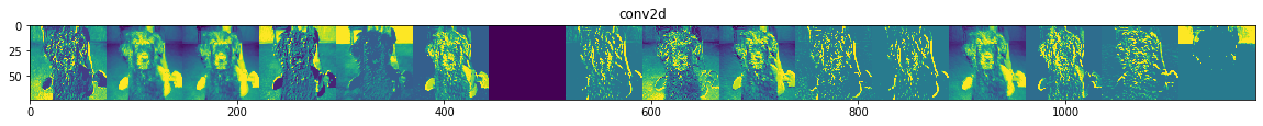

如上图片所示，我们得到从图像的原始像素到越来越抽象和紧凑的表示。下面的图像表示开始突出神经网络关注的内容，并且它们显示越来越少的特征被“激活”。

这些表示携带越来越少的关于图像原始像素的信息，但越来越精细的关于图像类别的信息。可以将神将网络模型视为图片信息的蒸馏管道，这样通过一层层的递进就得到了图像的较显著的特征。

评估模型精度与损失值

输出训练过程中随训练次数变化的精度与损失值的变化图

acc      = history.history[     'acc' ]val_acc  = history.history[ 'val_acc' ]loss     = history.history[    'loss' ]val_loss = history.history['val_loss' ]epochs   = range(len(acc))plt.plot  ( epochs,     acc ,label='acc')plt.plot  ( epochs, val_acc ,label='val_acc')plt.legend(loc='best')plt.title ('Training and validation accuracy')plt.figure()plt.plot  ( epochs,     loss ,label='loss')plt.plot  ( epochs, val_loss ,label='val_loss')plt.legend(loc='best')plt.title ('Training and validation loss')

通过观察图线发现出现了过拟合的现象，我们的训练准确度接近 100%，而我们的验证准确度停滞在大概70%。我们的验证损失值仅在五个epoch后就达到了最小值。

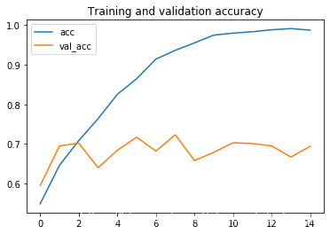
accuracy变化

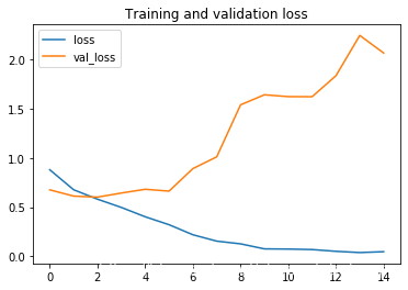
loss值变化

由于我们的训练样本数量相对较少，防止过度拟合应该是我们首要关注的问题。当训练数据过少，模型学习无法推广到新数据时，即当模型开始使用不相关的特征进行预测时，就会发生过度拟合。

感谢各位的阅读，以上就是“怎么利用Tensorflow2进行猫狗分类识别”的内容了，经过本文的学习后，相信大家对怎么利用Tensorflow2进行猫狗分类识别这一问题有了更深刻的体会，具体使用情况还需要大家实践验证。这里是亿速云，小编将为大家推送更多相关知识点的文章，欢迎关注！