Implement fashion_minst clothing image classification

 

活动地址：CSDN21天学习挑战赛

---

目录

1.跑通代码

2.代码分析

2.1

2.2

2.3

2.4

2.5

2.6

3.补充

---

Knowledge of some basic concepts in the text can be found in this article I wrote
(5条消息) tensorflow零基础入门学习_重邮研究森的博客-CSDN博客https://blog.csdn.net/m0_60524373/article/details/124143223

---

1.跑通代码

I am this guy for any code,I will go to run through the sum before watching the content,哈哈哈,So let's ignore it first37=21,Copy and paste a copy of the blogger's code directly to the running result.（PS：做了一些修改,Because the original isjupyter,而我在pycharm）

import tensorflow as tf
from tensorflow.keras import datasets, layers, models
import matplotlib.pyplot as plt
import numpy as np

(train_images, train_labels), (test_images, test_labels) = datasets.fashion_mnist.load_data()

# 将像素的值标准化至0到1的区间内.
train_images, test_images = train_images / 255.0, test_images / 255.0


#调整数据到我们需要的格式
train_images = train_images.reshape((60000, 28, 28, 1))
test_images = test_images.reshape((10000, 28, 28, 1))


class_names = ['T-shirt/top', 'Trouser', 'Pullover', 'Dress', 'Coat',
               'Sandal', 'Shirt', 'Sneaker', 'Bag', 'Ankle boot']

plt.figure(figsize=(20,10))
for i in range(20):
    plt.subplot(5,10,i+1)
    plt.xticks([])
    plt.yticks([])
    plt.grid(False)
    plt.imshow(train_images[i], cmap=plt.cm.binary)
    plt.xlabel(class_names[train_labels[i]])
plt.show()


model = models.Sequential([
    layers.Conv2D(32, (3, 3), activation='relu', input_shape=(28, 28, 1)),  # 卷积层1,卷积核3*3
    layers.MaxPooling2D((2, 2)),  # 池化层1,2*2采样
    layers.Conv2D(64, (3, 3), activation='relu'),  # 卷积层2,卷积核3*3
    layers.MaxPooling2D((2, 2)),  # 池化层2,2*2采样
    layers.Conv2D(64, (3, 3), activation='relu'),  # 卷积层3,卷积核3*3

    layers.Flatten(),  # Flatten层,连接卷积层与全连接层
    layers.Dense(64, activation='relu'),  # 全连接层,特征进一步提取
    layers.Dense(10)  # 输出层,输出预期结果
])
model.summary()  # 打印网络结构


model.compile(optimizer='adam',
              loss=tf.keras.losses.SparseCategoricalCrossentropy(from_logits=True),
              metrics=['accuracy'])

history = model.fit(train_images, train_labels, epochs=10,
                    validation_data=(test_images, test_labels))


plt.imshow(test_images[1])
plt.show()
#
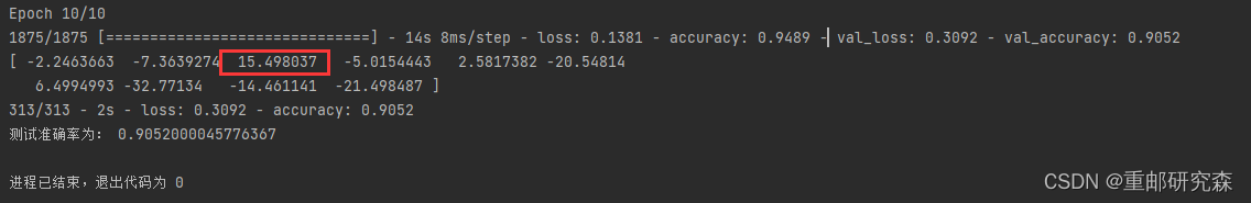
pre = model.predict(test_images) # 对所有测试图片进行预测
print( pre[1]) # Output the prediction result for the first image

plt.plot(history.history['accuracy'], label='accuracy')
plt.plot(history.history['val_accuracy'], label = 'val_accuracy')
plt.xlabel('Epoch')
plt.ylabel('Accuracy')
plt.ylim([0.5, 1])
plt.legend(loc='lower right')
plt.show()

test_loss, test_acc = model.evaluate(test_images,  test_labels, verbose=2)


print("测试准确率为：",test_acc)

点击pycharmThe final prediction result can be run！

 

2.代码分析

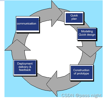
The whole process of the neural network is divided into the following six parts,And we will also analyze these six parts part by part.那么这6部分分别是：

六步法：

1->import

2->train test（指定训练集的输入特征和标签）

3->class MyModel(model) model=Mymodel（搭建网络结构,逐层描述网络）

4->model.compile（选择哪种优化器,损失函数）

5->model.fit（执行训练过程,输入训练集和测试集的特征+标签,batch,迭代次数）

6->验证

2.1

导入：这里很容易理解,That is, the various libraries needed to import the content of this experiment.This case mainly includes the following parts：

import tensorflow as tf
from tensorflow.keras import datasets, layers, models
import matplotlib.pyplot as plt
import numpy as np

主要是tensorflowand a library for drawing.

For this, we can copy and paste directly,When some other function is needed,Just add the corresponding library files.

2.2

设置训练集和测试集：The training of the neural network consists of two data sets,一个是训练集,一个是测试集.Among them, the training set data is more,The test set is small,Because training a model with more data, the relative model is more accurate.

The dataset in this paper takes advantage of the networkfashion_mnist数据集,The dataset is a dataset of clothes

The figure below shows the introduction of this dataset

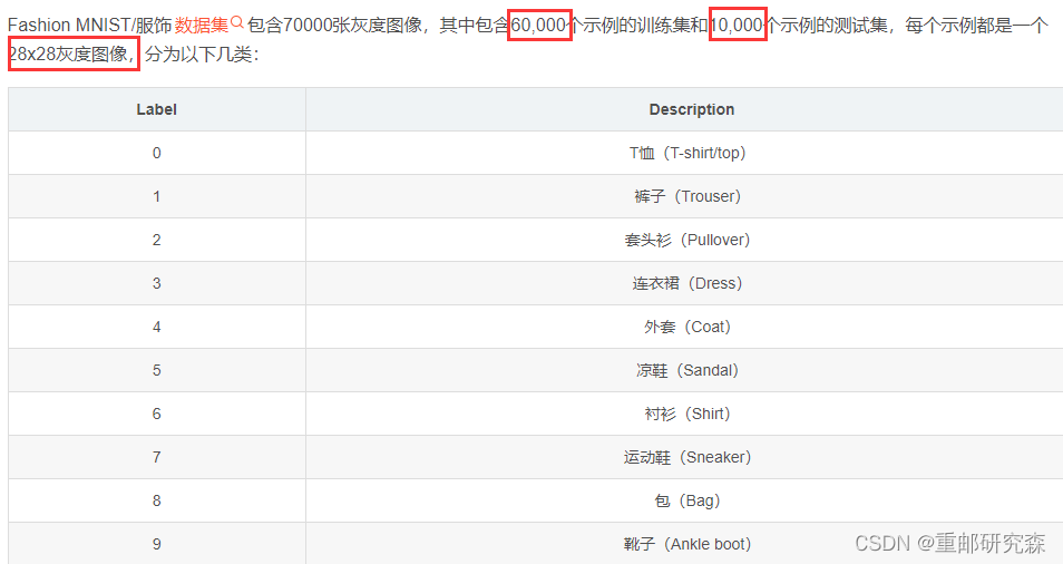
 注意事项：Since all the datasets in this experiment are image datasets,In order to make the network training results better,We need to normalize the image data.像素点是255个,So for data division255即可.

train_images, test_images = train_images / 255.0, test_images / 255.0

Normalized sum,Our image data still cannot be passed in directly,Input to the network model,We need to get the input data and network model“入口”保持一致.Therefore, we also need to resize the data,The size of the modification here is not clearly required.

train_images = train_images.reshape((60000, 28, 28, 1))
test_images = test_images.reshape((10000, 28, 28, 1))

注意事项：这里的60000和10000refers to the number of clothes in the dataset,28是指尺寸,而1is the number of channels in the gray image.

2.3

网络模型搭建：This is also the focus of neural networks！废话不多说,直接开始！

The structure diagram of the neural network in this paper is as follows：

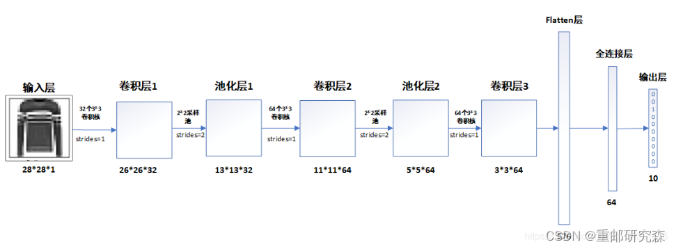
 在搭建模型的时候,We will follow this picture to build the model.

卷积层1：32通道,3x3尺寸,步长1的卷积核

 layers.Conv2D(32, (3, 3), activation='relu', input_shape=(28, 28, 1))

 注意事项：Here is the first layer of the network model,So add input

池化层1：The pooling layer is2x2

layers.MaxPooling2D((2, 2))

卷积层2：64通道,3x3尺寸,步长1的卷积核

 layers.Conv2D(64, (3, 3), activation='relu')

池化层2：The pooling layer is2x2

 layers.MaxPooling2D((2, 2))

卷积层3：64通道,3x3尺寸,步长1的卷积核

layers.Conv2D(64, (3, 3), activation='relu')

重点：

Now let's analyze how the dimension of the data after each layer in the picture comes from

经过卷积层1之后,原数据28x28变为26x26is because of a formula： （28-3）/stride+1=26

经过池化层1之后,原数据26x26变为13x13This is because the convolution kernel of the pooling pool is 2,所以13=26/2

经过卷积层2之后,原数据13变为11：如上,32变为64This is because the number of convolution kernel channels is 64

经过卷积层3之后,原数据（5-3）/stride+1=3

经过flatten层之后,数据数量=3*3*64=576

The output of the subsequent fully connected layer is set according to the fully connected layer code.The caveat is because the dataset is10种类型,因此最后为10

到此,We corresponded the reasons for the network model settings and the output results of the network model,We can see that the output of the network model is consistent with our analysis.

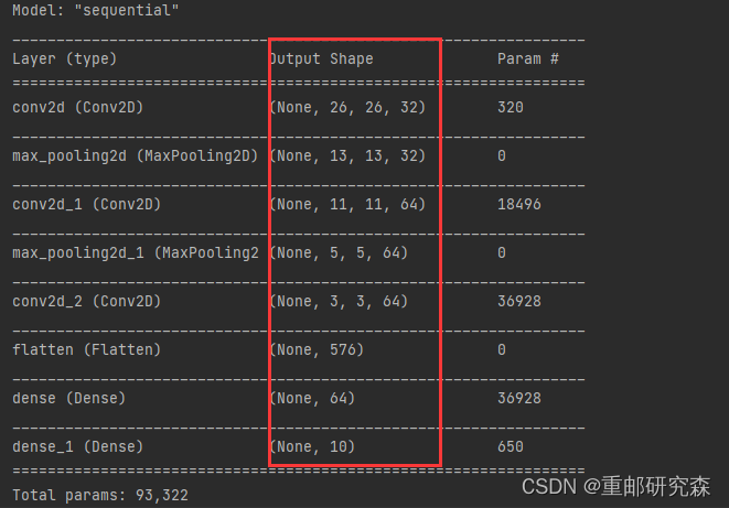
到此,We have finished analyzing the network model.

2.4

This part is just as important,It mainly completes the optimizer in the model training process,损失函数,Accuracy setting.

Let's take a look at this article.

model.compile(optimizer='adam',
              loss=tf.keras.losses.SparseCategoricalCrossentropy(from_logits=True),
              metrics=['accuracy'])

其中：For the meaning of these three contents, please refer to another basic blog post at the beginning of my article for a detailed introduction

2.5

This part is to perform the training,Then performing training definitely requires setting the training set data and its labels,Test set data and its labels,训练的epoch

history = model.fit(train_images, train_labels, epochs=10,
                    validation_data=(test_images, test_labels))

2.6

when the training is completed,We can take a test set or other data that meets the format for verification,这里为了方便,I use the test set to verify.

pre = model.predict(test_images) # 对所有测试图片进行预测
print( pre[1]) # Output the prediction result for the first image

3.补充

In this article we introduce some other concepts.模型评估

Take a look at the performance of our model with the accuracy curves on the training and testing sets.

plt.plot(history.history['accuracy'], label='accuracy')
plt.plot(history.history['val_accuracy'], label = 'val_accuracy')
plt.xlabel('Epoch')
plt.ylabel('Accuracy')
plt.ylim([0.5, 1])
plt.legend(loc='lower right')
plt.show()

test_loss, test_acc = model.evaluate(test_images,  test_labels, verbose=2)


print("测试准确率为：",test_acc)

Finally, we can get the model curve and the accuracy of the test set

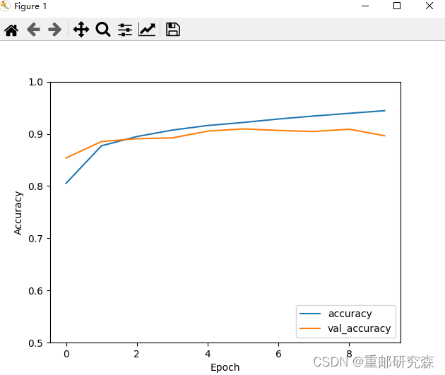
测试准确率为： 0.896399974822998