当前位置:网站首页>Deep learning: a solution to over fitting in deep neural networks
Deep learning: a solution to over fitting in deep neural networks
2022-07-02 01:51:00 【ShadyPi】
List of articles
L2 Regularization
With the Regularization in machine learning Agreement , Add the Frobenius norm of all weight matrices after the cost function , That is, the sum of the squares of all weight elements :
J ( W [ 1 ] , b [ 1 ] , ⋯ , W [ L ] , b [ L ] ) = 1 m ∑ i = 1 m L ( y ^ ( i ) , y ( i ) ) + λ 2 m ∑ l = 1 L ∣ ∣ W [ l ] ∣ ∣ F 2 ∣ ∣ W [ L ] ∣ ∣ F 2 = ∑ i = 1 n [ l ] ∑ j = 1 n [ l − 1 ] ( w i j [ l ] ) 2 J(W^{[1]},b^{[1]},\cdots,W^{[L]},b^{[L]})=\frac{1}{m}\sum_{i=1}^m\mathcal{L}(\hat{y}^{(i)},y^{(i)})+\frac{\lambda}{2m}\sum_{l=1}^L||W^{[l]}||^2_F\\ ||W^{[L]}||^2_F=\sum_{i=1}^{n^{[l]}}\sum_{j=1}^{n^{[l-1]}}(w_{ij}^{[l]})^2 J(W[1],b[1],⋯,W[L],b[L])=m1i=1∑mL(y^(i),y(i))+2mλl=1∑L∣∣W[l]∣∣F2∣∣W[L]∣∣F2=i=1∑n[l]j=1∑n[l−1](wij[l])2
Finally, the expression of gradient is the same as machine learning regularization , Added a λ m w \frac{\lambda}{m}w mλw, So the formula of backward propagation is changed to
d Z [ l ] = d A [ l ] ∗ g [ l ] ′ ( Z [ l ] ) d W [ l ] = 1 m d Z [ l ] A [ l − 1 ] T + λ m d W [ l ] d b [ l ] = 1 m n p . s u m ( d Z [ l ] , a x i s = 1 , k e e p d i m s = T r u e ) d A [ l − 1 ] = W [ l ] T d Z [ l ] \begin{aligned} &dZ^{[l]}=dA^{[l]}*g^{[l]'}(Z^{[l]})\\ &dW^{[l]}=\frac{1}{m}dZ^{[l]}A^{[l-1]T}+\frac{\lambda}{m}dW^{[l]}\\ &db^{[l]}=\frac{1}{m}np.sum(dZ^{[l]},axis=1,keepdims=True)\\ &dA^{[l-1]}=W^{[l]T}dZ^{[l]} \end{aligned} dZ[l]=dA[l]∗g[l]′(Z[l])dW[l]=m1dZ[l]A[l−1]T+mλdW[l]db[l]=m1np.sum(dZ[l],axis=1,keepdims=True)dA[l−1]=W[l]TdZ[l]
The principle is probably by adding norms to the cost function , Make the algorithm try to reduce the weight ( near 0), Equivalent to reducing the influence of hidden nodes , And fewer hidden nodes , The model will change from high square error to high deviation , When you have a suitable λ \lambda λ You can get a reasonable model .
Why not add about the offset matrix b b b Regularization of ? It's because of the comparison W W W, b b b The number of elements is very small , So the value of its Frobenius norm is compared W W W It's also very small , In the cost function, we get “ Focus on ” Still W W W The elements in , and b b b Whether you participate in regularization or not doesn't matter much , So we won't waste time .
The disadvantage is to debug parameters λ \lambda λ, It needs repeated training .
Random deactivation (dropout)
Random deactivation refers to every training , Make some nodes fail randomly , Delete all paths connected to these nodes , Carry out forward propagation and back propagation on this network to train the model .
A common implementation is reverse random deactivation , For the first l l l Node vectors of hidden layers a [ l ] a^{[l]} a[l], We generate a random vector of the same size , The value of each element is [ 0 , 1 ] [0,1] [0,1]. For elements less than the set threshold, set to 1, Greater than is set to 0, Use this vector and a [ l ] a^{[l]} a[l] Element corresponding multiplication , You can reset some nodes randomly . The set threshold is called keep-prob, That is, the probability of retaining nodes .
Set the node 0 after , For the remaining nodes , We have to divide 1/keep-prob. Because the expectation of output will become original after setting zero keep-prob times , In order to keep the output expectation unchanged ( This is very helpful in testing ), We need to divide keep-prob.
In the actual test , We don't need to randomly disable nodes anymore , Directly operate according to the normal forward propagation , Because when we train, we have made the expectation of the output of the whole model unchanged .
The reason why random deactivation regularization is effective , Because it is equivalent to every training on a smaller neural network , Small scale networks are not easy to fit . meanwhile , Because every node can be set to zero , So the model will not depend on a certain eigenvalue , Instead, we will try to integrate all the information spread .
in addition , Threshold of each layer keep-prob It can be different , For some hidden layers with a large number of nodes , They are more likely to be fitted , We will take keep-prob Set it smaller , Those that are not easy to fit can be larger , It can even be set to 1 Keep it all . But then there are more super parameters ……
Another disadvantage is that after using random deactivation , There is no well-defined cost function , If the cost function is forcibly drawn - Iteration number image , The curve is probably not simply subtracted .
Dataset expansion
Simply speaking , Is to use a larger training set , In this way, there will be no over fitting , If you can't collect data , You can add some magic changes to the existing data .
Early termination method
Simply speaking , That is to stop training directly in the process of the model gradually being trained from high deviation to high variance , If the time to stop is clever enough , We can get a good model . A scientific judgment method draws the cost function curve of the verification set , Stop at the lowest cost of the validation set .
The advantage of this method is that there are no super parameters to debug , We just need to look at the lowest value of the cost function of the verification set in the first few iterations , Then restart the training and stop the training at the corresponding iteration number , It's very simple and fast . The disadvantage is that this method mixes the two tasks of reducing the value of the cost function and avoiding over fitting , It violates the idea of orthogonalization ( One module only does one thing ), Sometimes it makes things complicated .
边栏推荐
- 1218 square or round
- Parted command
- 电商系统中常见的9大坑,你踩过没?
- II Basic structure of radio energy transmission system
- Niuke - Huawei question bank (51~60)
- Construction and maintenance of business websites [13]
- Based on configured schedule, the given trigger will never fire
- 卷积神经网络(包含代码与相应图解)
- Self drawing of menu items and CListBox items
- 10 minutes to get started quickly composition API (setup syntax sugar writing method)
猜你喜欢

ES6 new method of string

遷移雲計算工作負載的四個基本策略

三分钟学会基础k线图知识
1222. Password dropping (interval DP, bracket matching)

MySQL如何解决delete大量数据后空间不释放的问题

Réseau neuronal convolutif (y compris le Code et l'illustration correspondante)

5g/4g pole gateway_ Smart pole gateway
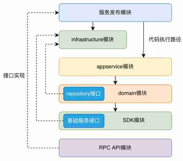
Architecture evolution from MVC to DDD
![[Video] Markov chain Monte Carlo method MCMC principle and R language implementation | data sharing](/img/ba/dcb276768b1a9cc84099f093677d29.png)
[Video] Markov chain Monte Carlo method MCMC principle and R language implementation | data sharing
【视频】马尔可夫链蒙特卡罗方法MCMC原理与R语言实现|数据分享
随机推荐
【LeetCode 43】236. The nearest common ancestor of binary tree
New news, Wuhan Yangluo international port, filled with black technology, refreshes your understanding of the port
Architecture evolution from MVC to DDD
Experimental reproduction of variable image compression with a scale hyperprior
Raspberry pie 4B learning notes - IO communication (1-wire)
The role of artificial intelligence in network security
This is the form of the K-line diagram (pithy formula)
[Floyd] post disaster reconstruction
Based on configured schedule, the given trigger will never fire
Using tabbar in wechat applet
1217 supermarket coin processor
Medical management system (C language course for freshmen)
Laravel artisan 常用命令
Bat Android Engineer interview process analysis + restore the most authentic and complete first-line company interview questions
Android high frequency network interview topic must know and be able to compare Android development environment
I Brief introduction of radio energy transmission technology
[rust web rokcet Series 2] connect the database and add, delete, modify and check curd
Volume compression, decompression
现货黄金分析的技巧有什么呢?
微信小程序中使用tabBar