Call pytorch API to complete linear regression

Pytorch Complete the basic model

The goal is

1. know Pytorch in Module How to use
2. know Pytorch How to use the optimizer class in
3. know Pytorch The common use of loss function in
4. Know how to GPU Run code on
5. Be able to say common optimizers and their principles

1. Pytorch Complete the model API

In the previous part , We achieved it ourselves through torch Back propagation and parameter updating are completed by the relevant methods of , stay pytorch Some more flexible and simple objects are preset in , Let's construct the model 、 Define loss , Optimization loss, etc

So next , Let's take a look at the commonly used API

1.1 nn.Module

nn.Modul yes torch.nn A class provided , yes pytorch We Custom network A base class of , There are many useful methods defined in this class , Let's inherit this class and define the network very simply

When we customize the network , There are two ways to pay special attention ：

1. __init__ Need to call super Method , Inherits the properties and methods of the parent class
2. farward Method must implement , The process used to define the forward computation of our network

Use the front one y = wx+b An example of the model is as follows ：

from torch import nn
class Lr(nn.Module):
    def __init__(self):
        super(Lr, self).__init__()  # Inherited parent class init Parameters of 
        self.linear = nn.Linear(1, 1) 

    def forward(self, x):
        out = self.linear(x)
        return out

Be careful ：

1. nn.Linear by torch Predefined linear model , Also known as Full link layer , The parameter passed in is the number of inputs , Number of outputs (in_features, out_features), It doesn't count (batch_size Columns of )
2. nn.Module Defined __call__ Method , The implementation is to call forward Method , namely Lr Example , Can be called directly by passed in parameters , It's actually calling theta forward Method and pass in parameters

#  Instantiation model 
model = Lr()
#  Incoming data , The result of the calculation is 
predict = model(x)

1.2 Optimizer class

Optimizer (optimizer), It can be understood as torch The method encapsulated for us to update parameters , For example, the common random gradient descent (stochastic gradient descent,SGD)

Optimizer classes are composed of torch.optim Provided , for example

1. torch.optim.SGD( Parameters , Learning rate )
2. torch.optim.Adam( Parameters , Learning rate )

Be careful ：

1. Parameters can be used model.parameters() To get , Get all the data in the model requires_grad=True Parameters of
2. Optimize the use of classes
   1. Instantiation
   2. Gradient of all parameters , Set the value to 0
   3. Back propagation calculation gradient
   4. Update parameter values

Examples are as follows ：

optimizer = optim.SGD(model.parameters(), lr=1e-3) #1.  Instantiation 
optimizer.zero_grad() #2.  Set the gradient to 0
loss.backward() #3.  Calculate the gradient 
optimizer.step()  #4.  Update the value of the parameter 

1.3 Loss function

The previous example is a regression problem ,torch Many loss functions are also predicted in

1. Mean square error :nn.MSELoss(), Often used in regression problems
2. Cross entropy loss ：nn.CrossEntropyLoss(), Commonly used for classification problems

Usage method ：

model = Lr() #1.  Instantiation model 
criterion = nn.MSELoss() #2.  Instantiate the loss function 
optimizer = optim.SGD(model.parameters(), lr=1e-3) #3.  Instantiate the optimizer class 
for i in range(100):
    y_predict = model(x_true) #4.  Calculate the predicted value forward 
    loss = criterion(y_true,y_predict) #5.  Call the loss function to pass in the real value and the predicted value , Get the loss result 
    optimizer.zero_grad() #5.  The current loop parameter gradient is set to 0
    loss.backward() #6.  Calculate the gradient 
    optimizer.step()  #7.  Update the value of the parameter 

1.4 Complete the linear regression code

import torch
from torch import nn
from torch import optim
import numpy as np
from matplotlib import pyplot as plt

# 1.  Defining data 
x = torch.rand([50,1])
y = x*3 + 0.8

#2 . Defining models 
class Lr(nn.Module):
    def __init__(self):
        super(Lr,self).__init__()
        self.linear = nn.Linear(1,1)
		
    def forward(self, x):
        out = self.linear(x)
        return out

# 2.  Instantiation model ,loss, And optimizer 
model = Lr()
criterion = nn.MSELoss()
optimizer = optim.SGD(model.parameters(), lr=1e-3)
#3.  Training models 
for i in range(30000):
    out = model(x) #3.1  Get predictions 
    loss = criterion(y,out) #3.2  Calculate the loss 
    optimizer.zero_grad()  #3.3  The gradient goes to zero 
    loss.backward() #3.4  Calculate the gradient 
    optimizer.step()  # 3.5  Update gradient 
    if (i+1) % 20 == 0:
        print('Epoch[{}/{}], loss: {:.6f}'.format(i,30000,loss.data))

#4.  Model to evaluate 
model.eval() # Set the model to evaluation mode , Prediction mode 
predict = model(x)
predict = predict.data.numpy()
plt.scatter(x.data.numpy(),y.data.numpy(),c="r")
plt.plot(x.data.numpy(),predict)
plt.show()

Output is as follows ：

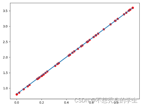
Be careful ：

model.eval() Indicates that the model is set to the evaluation mode , Prediction mode

model.train(mode=True) Indicates that the model is set to training mode

In the current linear regression , There is no difference between the above

But in other models , The parameters of training and prediction will be different , At that time, we need to tell the program whether we are training or predicting , For example, there are Dropout,BatchNorm When

2. stay GPU Run code on

When the model is too large , Or when there are too many parameters , To speed up your training , Often use GPU To train

At this point, our code needs to be adjusted slightly ：

1. Judge GPU Is it available torch.cuda.is_available()

   torch.device("cuda:0" if torch.cuda.is_available() else "cpu")
   >>device(type='cuda', index=0)  # Use gpu
   >>device(type='cpu') # Use cpu
   

2. Compare the model parameters with input Data into cuda Type of support for

   model.to(device)
   x_true.to(device)
   

3. stay GPU The calculation result is also cuda Data type of , We need to convert to numpy perhaps torch Of cpu Of tensor type

   predict = predict.cpu().detach().numpy() 
   

   detach() The effect and data Similarity of , however detach() It's a deep copy ,data It's a value , Is a shallow copy

The modified code is as follows ：

import torch
from torch import nn
from torch import optim
import numpy as np
from matplotlib import pyplot as plt
import time

# 1.  Defining data 
x = torch.rand([50,1])
y = x*3 + 0.8

#2 . Defining models 
class Lr(nn.Module):
    def __init__(self):
        super(Lr,self).__init__()
        self.linear = nn.Linear(1,1)

    def forward(self, x):
        out = self.linear(x)
        return out

# 2.  Instantiation model ,loss, And optimizer 

device = torch.device("cuda:0" if torch.cuda.is_available() else "cpu")
x,y = x.to(device),y.to(device)

model = Lr().to(device)
criterion = nn.MSELoss()
optimizer = optim.SGD(model.parameters(), lr=1e-3)

#3.  Training models 
for i in range(300):
    out = model(x)
    loss = criterion(y,out)

    optimizer.zero_grad()
    loss.backward()
    optimizer.step()
    if (i+1) % 20 == 0:
        print('Epoch[{}/{}], loss: {:.6f}'.format(i,30000,loss.data))

#4.  Model to evaluate 
model.eval() #
predict = model(x)
predict = predict.cpu().detach().numpy() # Turn into numpy Array 
plt.scatter(x.cpu().data.numpy(),y.cpu().data.numpy(),c="r")
plt.plot(x.cpu().data.numpy(),predict,)
plt.show()

3. Introduction to common optimization algorithms

3.1 Gradient descent algorithm （batch gradient descent BGD）

Each iteration needs to send all samples into , The advantage is that each iteration takes into account all the samples , What we do is global optimization , But it is possible to achieve local optimization .

3.2 Random gradient descent method (Stochastic gradient descent SGD)

Aiming at the disadvantage that the training speed of gradient descent algorithm is too slow , A stochastic gradient descent algorithm is proposed , Random gradient descent algorithm is to randomly extract a group of samples , Update once according to the gradient after training , Then take another group , Update again , When the sample size is extremely large , It may not be necessary to train all the samples to obtain a model with a loss value within an acceptable range .

torch Medium api by ：torch.optim.SGD()

3.3 Small batch gradient descent (Mini-batch gradient descent MBGD）

SGD It's much faster , But there are also problems , Because the training of a single sample may bring a lot of noise , bring SGD It's not going to be optimization every time , Therefore, it may converge quickly at the beginning of training , But after training for a period of time, it will become very slow . On this basis, a small batch gradient descent method is proposed , It is to randomly select a small batch of samples for training each time , Not a group , This ensures both the effect and the speed .

3.4 Momentum method

mini-batch SGD Although this algorithm can bring good training speed , But when you reach the best, you can't always really reach the best , But hovering around the best .

Another drawback is mini-batch SGD We need to choose an appropriate learning rate , When we use a small learning rate , It will cause the network to converge too slowly during training ; When we adopt a large learning rate , It will cause the amplitude optimized during training to skip the range of the function , That is, it is possible to skip the best . What we hope is that when the network is optimized, the loss function of the network has a good convergence speed and does not swing too much .

therefore Momentum The optimizer can just solve the problem we face , It is mainly a moving exponential weighted average based on gradient , Smoothing the gradient of the network , Make the swing amplitude of the gradient smaller .

\begin{align*}
&gradent = 0.8\nabla w + 0.2 history_gradent &,\nabla w Represents the current gradient \
&w = w - \alpha* gradent &,\alpha It means the learning rate
\end{align*}

（ notes ：t+1 Of course histroy_gradent For the first time t Time of gradent）

3.5 AdaGrad

AdaGrad The algorithm is to square the gradient of each iteration of each parameter and accumulate it in the square , Divide the global learning rate by this number , As a dynamic update of learning rate , So as to achieve Adaptive learning rate The effect of

\begin{align*}
&gradent = history_gradent + (\nabla w)^2 \
&w = w - \frac{\alpha}{\sqrt{gradent}+\delta} \nabla w ,&\delta Is a small constant , For numerical stability, set to approximately 10^{-7}
\end{align*}

3.6 RMSProp

Momentum In the optimization algorithm , Although the problem of large swing range in optimization is preliminarily solved , In order to further optimize the loss function, there is a problem that the swing amplitude is too large , And further accelerate the convergence speed of the function ,RMSProp The algorithm uses the square weighted average for the gradient of parameters .

\begin{align*}
& gradent = 0.8history_gradent + 0.2(\nabla w)^2 \
& w = w - \frac{\alpha}{\sqrt{gradent}+\delta} \nabla w
\end{align*}

3.7 Adam

Adam（Adaptive Moment Estimation） The algorithm is to Momentum Algorithm and RMSProp An algorithm used in combination with algorithms , How much swing can be achieved to prevent gradient , At the same time, it can also increase the convergence rate

\begin{align*}
& 1. You need to initialize the cumulant and square cumulant of the gradient \
& v_w = 0,s_w = 0 \
& 2. The first t In round training , We can first calculate Momentum and RMSProp Parameter update for ：\
& v_w = 0.8v + 0.2 \nabla w \qquad,Momentum Calculated gradient \
& s_w = 0.8s + 0.2(\nabla w)^2 \qquad,RMSProp Calculated gradient \
& 3. After processing the values , obtain ：\
& w = w - \frac{\alpha}{\sqrt{s_w}+\delta} v_w
\end{align*}

torch Medium api by ：torch.optim.Adam()

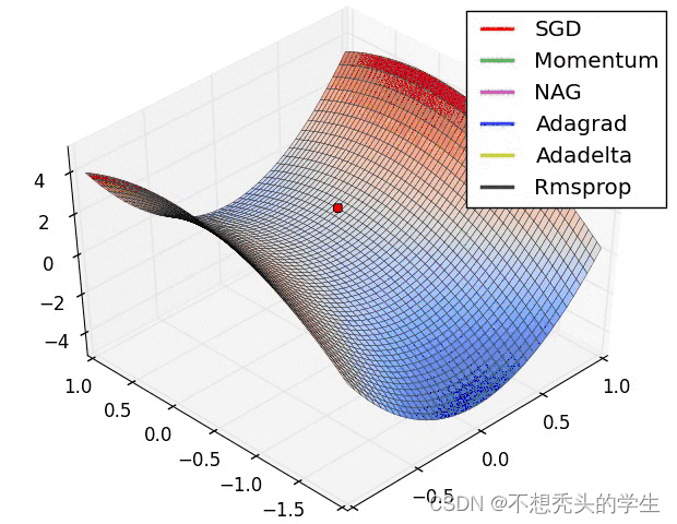
3.8 Effect demonstration ：

It can be calculated that Momentum and RMSProp Parameter update for ：\
& v_w = 0.8v + 0.2 \nabla w \qquad,Momentum Calculated gradient \
& s_w = 0.8s + 0.2(\nabla w)^2 \qquad,RMSProp Calculated gradient \
& 3. After processing the values , obtain ：\
& w = w - \frac{\alpha}{\sqrt{s_w}+\delta} v_w
\end{align*}
$$
torch Medium api by ：torch.optim.Adam()

3.8 Effect demonstration ：

​