当前位置:网站首页>Wu Enda's machine learning after class exercises - linear regression
Wu Enda's machine learning after class exercises - linear regression
2022-07-26 04:15:00 【Yizhou YZ】
Univariate linear regression
import numpy as np
import pandas as pd
import matplotlib.pyplot as plt
path = "ex1data1.txt"
data = pd.read_csv(path, header=None, names=['Population', 'Profit'])
# pandas.read_csv By default, the first row of the data content will be defaulted to the field name Title ,header=None Indicates that the read raw file data has no column index
data.head() #  Method is used to return the first... Of a data frame or sequence n That's ok ( The default value is 5). Return type :DataFrame, It can be understood as a table , Or matrix
# DataFrame It is essentially a two-dimensional matrix , The difference from the conventional two-dimensional matrix is that the former additionally specifies the names of each row and column .
| Population | Profit | |
|---|---|---|
| 0 | 6.1101 | 17.5920 |
| 1 | 5.5277 | 9.1302 |
| 2 | 8.5186 | 13.6620 |
| 3 | 7.0032 | 11.8540 |
| 4 | 5.8598 | 6.8233 |
data.describe()
# describe()  Function can view the basic situation of data ,
#  Include :count  Non null number 、mean  Average 、std  Standard deviation 、max  Maximum 、min  minimum value 、(25%、50%、75%) Quantiles, etc. .
| Population | Profit | |
|---|---|---|
| count | 97.000000 | 97.000000 |
| mean | 8.159800 | 5.839135 |
| std | 3.869884 | 5.510262 |
| min | 5.026900 | -2.680700 |
| 25% | 5.707700 | 1.986900 |
| 50% | 6.589400 | 4.562300 |
| 75% | 8.578100 | 7.046700 |
| max | 22.203000 | 24.147000 |
#  Draw a picture
data.plot(kind='scatter',x='Population',y='Profit',figsize=(12,8))
# scatter Represents a scatter plot ,figsize Show the size of the picture , Company : Inch
plt.show()

Use gradient descent to minimize the cost function ,
Create a parameter to θ Is the cost function of the characteristic function
J ( θ ) = 1 2 m ∑ i = 1 m ( h θ ( x ( i ) ) − y ( i ) ) 2 J\left( \theta \right)=\frac{1}{2m}\sum\limits_{i=1}^{m}{ { {\left( { {h}_{\theta }}\left( { {x}^{(i)}} \right)-{ {y}^{(i)}} \right)}^{2}}} J(θ)=2m1i=1∑m(hθ(x(i))−y(i))2
among :
h θ ( x ) = θ T X = θ 0 x 0 + θ 1 x 1 + θ 2 x 2 + . . . + θ n x n { {h}_{\theta }}\left( x \right)={ {\theta }^{T}}X={ {\theta }_{0}}{ {x}_{0}}+{ {\theta }_{1}}{ {x}_{1}}+{ {\theta }_{2}}{ {x}_{2}}+...+{ {\theta }_{n}}{ {x}_{n}}\\ hθ(x)=θTX=θ0x0+θ1x1+θ2x2+...+θnxn
def computeCost(X,y,theta): #  Input X Is a column vector ,y It's also a column vector ,theta It's a line vector
    inner = np.power(((X*theta.T)-y),2) # x*θ The transpose of is a hypothetical function  power Function calculation numpy The specified power of each value in the array
    return np.sum(inner/(2*len(X))) #  Will array / All the elements in the matrix add up  len(X) Number of matrix lines
data.insert(0,'Ones',1)
#  Insert a column as 1 For better vectorization , You need to add a column to the training set x_0, So that we can use the vectorized solution to calculate the cost and gradient , See video p18
#  Initialization of a variable
cols = data.shape[1] # shape[0] It's the number of lines  shape[1] It's the number of columns
X = data.iloc[:,0:cols-1] #  Data sets   All right   List from 0 To cols-1( barring )  Left closed right away
y = data.iloc[:,cols-1:cols] #  The target
X.head()
| Ones | Population | |
|---|---|---|
| 0 | 1 | 6.1101 |
| 1 | 1 | 5.5277 |
| 2 | 1 | 8.5186 |
| 3 | 1 | 7.0032 |
| 4 | 1 | 5.8598 |
The data type obtained is DataFrame type , So you need to do type conversion . Initialization is also required theta, namely theta All elements are set to 0
X = np.matrix(X.values)
y = np.matrix(y.values)
theta = np.matrix(np.array([0,0]))
dimension
X.shape, theta.shape, y.shape
((97, 2), (1, 2), (97, 1))
computeCost(X,y,theta) # Computational cost function
32.072733877455676
batch gradient decent( Batch gradient descent )
θ j : = θ j − α ∂ ∂ θ j J ( θ ) { {\theta }_{j}}:={ {\theta }_{j}}-\alpha \frac{\partial }{\partial { {\theta }_{j}}}J\left( \theta \right) θj:=θj−α∂θj∂J(θ)
gradient descent
def gradientDescent(X,y,theta,alpha,iters): # iters Is the number of iterations  alpha It's the learning rate   That is, step length
    temp_theta = np.matrix(np.zeros(theta.shape)) #  Zero value matrix   The staging theta
    parameters = int(theta.ravel().shape[1]) # ravel Calculate the number of parameters to be solved   Function reduces multidimensional array to one dimension   The value here is 2
    cost = np.zeros(iters) # structure iters individual 0 Array of
    # iteration :
    for i in range(iters):
        difference = (X*theta.T) - y #  Difference value
        for j in range(parameters):
            term = np.multiply(difference,X[:,j])    # multiply x_i X[:,j] Represents all lines  j Column , In short, draw out the number j Column
             #  Note that this is not matrix multiplication   Here is the multiplication after derivation  multiply Is the number of corresponding positions of two matrices of the same size multiplied directly
            temp_theta[0,j] = theta[0,j] - (alpha/len(X))*np.sum(term) #  to update theta_j

        theta = temp_theta #  Update all theta value
        cost[i] = computeCost(X,y,theta) #  Renewal value

    return theta,cost
Initialize some additional variables - Learning rate α And the number of iterations to perform .
alpha = 0.01
iters = 1000
obtain theta value , Minimum cost
g,cost = gradientDescent(X,y,theta,alpha,iters)
g
matrix([[-3.24140214, 1.1272942 ]])
cost[-1] # Get the last value of the array
4.515955503078913
Last , Use what we fitted theta Value calculation of the cost function of the training model
computeCost(X, y, g)
4.515955503078913
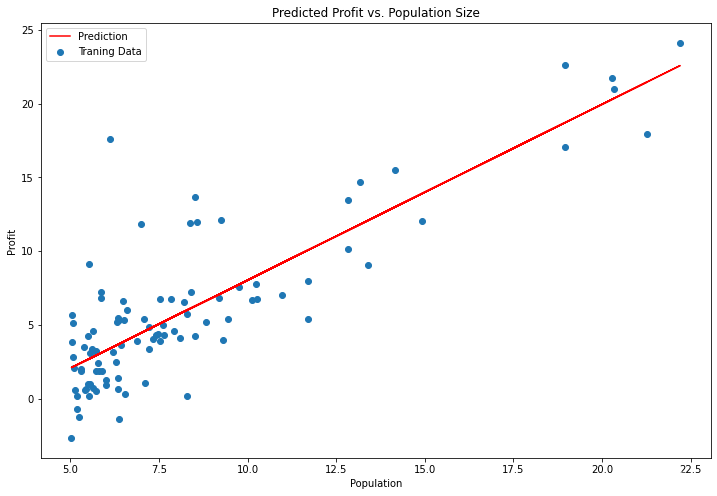
Draw linear models and data , Intuitively see its fitting
x = np.linspace(data.Population.min(), data.Population.max(), 100) #  Generates a one-dimensional array of the specified number within the specified range
f = g[0, 0] + (g[0, 1] * x) # x1=1 g[0, 0] Express theta_0 g[0, 1] Express theta_1

fig, ax = plt.subplots(figsize=(12,8)) # plt.subplot() Function is used to directly specify the division method and position for drawing .
# fig Represents the drawing window (Figure);ax Represents the coordinate system on this drawing window (axis), Will generally continue to ax To operate .

#  Function to set the abscissa and ordinate , And set the color to red , Mark... On the icon 'Prediction' label   Abscissa x  Ordinate f
ax.plot(x, f, 'r', label='Prediction')
#  Define the abscissa and ordinate of the scatter chart , The of scatter plot points is given 'Traning Data' Tag name
ax.scatter(data.Population, data.Profit, label='Traning Data')
ax.legend(loc=2)  # 2 In the upper left corner


ax.set_xlabel('Population')
ax.set_ylabel('Profit')
ax.set_title('Predicted Profit vs. Population Size')
plt.show()

Since the gradient equation function also outputs a cost vector in each training iteration , So we can also draw . Be careful , The cost is always lower
fig, ax = plt.subplots(figsize=(12,8))
ax.plot(np.arange(iters), cost, 'r')
ax.set_xlabel('Iterations')
ax.set_ylabel('Cost')
ax.set_title('Error vs. Training Epoch')
plt.show()

Multivariate linear regression
This exercise includes a housing price data set , It contains two variables ( The size of the house 、 Number of bedrooms ) And the target ( House price ).
path =  'ex1data2.txt'
data2 = pd.read_csv(path, header=None, names=['Size', 'Bedrooms', 'Price'])
data2.head()
| Size | Bedrooms | Price | |
|---|---|---|---|
| 0 | 2104 | 3 | 399900 |
| 1 | 1600 | 3 | 329900 |
| 2 | 2400 | 3 | 369000 |
| 3 | 1416 | 2 | 232000 |
| 4 | 3000 | 4 | 539900 |
data2.describe()
| Size | Bedrooms | Price | |
|---|---|---|---|
| count | 47.000000 | 47.000000 | 47.000000 |
| mean | 2000.680851 | 3.170213 | 340412.659574 |
| std | 794.702354 | 0.760982 | 125039.899586 |
| min | 852.000000 | 1.000000 | 169900.000000 |
| 25% | 1432.000000 | 3.000000 | 249900.000000 |
| 50% | 1888.000000 | 3.000000 | 299900.000000 |
| 75% | 2269.000000 | 4.000000 | 384450.000000 |
| max | 4478.000000 | 5.000000 | 699900.000000 |
The house is about the size of the number of bedrooms 1000 times . When features differ by several orders of magnitude , First perform feature scaling ( Mean normalization ) It can make the gradient descent converge faster .
data2 = (data2 - data2.mean()) / data2.std() #  The solution is to try to scale all feature scales to  -1 ~ 1
data2.head()
| Size | Bedrooms | Price | |
|---|---|---|---|
| 0 | 0.130010 | -0.223675 | 0.475747 |
| 1 | -0.504190 | -0.223675 | -0.084074 |
| 2 | 0.502476 | -0.223675 | 0.228626 |
| 3 | -0.735723 | -1.537767 | -0.867025 |
| 4 | 1.257476 | 1.090417 | 1.595389 |
data2.insert(0, 'Ones', 1)
cols = data2.shape[1]
X2 = data2.iloc[:,0:cols-1]
y2 = data2.iloc[:,cols-1:cols]

X2 = np.matrix(X2.values)
y2 = np.matrix(y2.values)
theta2 = np.matrix(np.array([0,0,0]))
g2, cost2 = gradientDescent(X2, y2, theta2, alpha, iters)
computeCost(X2, y2, g2) #  Calculate the cost
0.1307033696077189
Cost function convergence graph
fig, ax = plt.subplots(figsize=(12,8))
ax.plot(np.arange(iters), cost2, 'r')
ax.set_xlabel('Iterations')
ax.set_ylabel('Cost')
ax.set_title('Error vs. Training Epoch')
plt.show()

Use sklearn Linear regression function simplification process
from sklearn import linear_model
model = linear_model.LinearRegression()  # Linear regression based on least square method .
model.fit(X, y)
x = np.array(X[:, 1].A1)
f = model.predict(X).flatten()

fig, ax = plt.subplots(figsize=(12,8))
ax.plot(x, f, 'r', label='Prediction')
ax.scatter(data.Population, data.Profit, label='Traning Data')
ax.legend(loc=2)
ax.set_xlabel('Population')
ax.set_ylabel('Profit')
ax.set_title('Predicted Profit vs. Population Size')
plt.show()
normal equation( Normal equation )
Ideas
The normal equation is to find the parameters that minimize the cost function by solving the following equation : ∂ ∂ θ j J ( θ j ) = 0 \frac{\partial }{\partial { {\theta }_{j}}}J\left( { {\theta }_{j}} \right)=0 ∂θj∂J(θj)=0 .
Suppose that the characteristic matrix of our training set is X( Contains x 0 = 1 { {x}_{0}}=1 x0=1) And the result of our training set is vector y, Then use the normal equation to solve the vector θ = ( X T X ) − 1 X T y \theta ={ {\left( { {X}^{T}}X \right)}^{-1}}{ {X}^{T}}y θ=(XTX)−1XTy .
Superscript T Transposition of representative matrix , Superscript -1 Represents the inverse of a matrix . Let's set the matrix A = X T X A={ {X}^{T}}X A=XTX, be : ( X T X ) − 1 = A − 1 { {\left( { {X}^{T}}X \right)}^{-1}}={ {A}^{-1}} (XTX)−1=A−1
Gradient descent versus normal equation :
gradient descent : We need to choose the learning rate α, It takes several iterations , When the number of features n It can also be better applied when it is large , It's suitable for all kinds of models
Normal equation : There is no need to choose the learning rate α, Calculated at one time , Need to compute ( X T X ) − 1 { {\left( { {X}^{T}}X \right)}^{-1}} (XTX)−1, If the number of features n If it's bigger, it's more expensive , Because the computation time complexity of matrix inverse is O ( n 3 ) O(n3) O(n3), Generally speaking, when n n n Less than 10000 It's still acceptable , Only for linear models , It is not suitable for other models such as logistic regression model
#  Normal equation function
def normalEqn(X, y):
    theta = np.linalg.inv(X.[email protected])@X.[email protected]#[email protected] Equivalent to X.T.dot(X) np.linalg.inv(): Matrix inversion
    return theta
final_theta2=normalEqn(X, y)
final_theta2  #  gradient matrix([[-3.24140214, 1.1272942 ]])
matrix([[-3.89578088],
        [ 1.19303364]])
边栏推荐
- How to download the supplementary literature?
- 生活相关——十年的职业历程(转)
- Under the high debt of Red Star Macalline, is it eyeing new energy?
- Acwing game 61 [End]
- [question 019: what is the understanding of spherecastcommand in unity?]
- Operator new, operator delete supplementary handouts
- Synchronous FIFO based on shift register
- Life related - less expectation, happier
- In PHP, you can use the abs() function to turn negative numbers into positive numbers
- Can literature | relationship research draw causal conclusions
猜你喜欢

PathMatchingResourcePatternResolver解析配置文件 资源文件
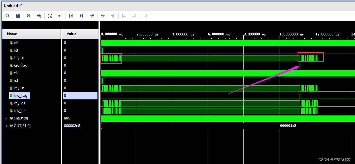
Verilog implementation of key dithering elimination

Chapter 18: explore the wonders of the mean in the 2-bit a~b system, specify the 3x+1 conversion process of integers, specify an interval to verify the angular Valley conjecture, explore the number of

Acwing刷题
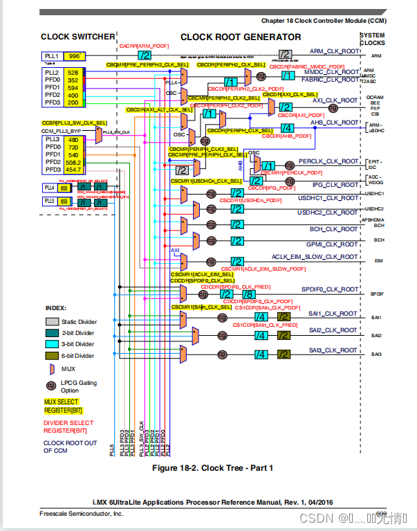
I.MX6U-ALPHA开发板(主频和时钟配置实验)

综合评价与决策方法

荐书|《DBT技巧训练手册》:宝贝,你就是你活着的原因

Life related - ten years of career experience (turn)

苹果在其产品中拿掉了最后一颗Intel芯片

Wechat applet to realize music player (4) (use pubsubjs to realize inter page communication)
随机推荐
Yadi started to slow down after high-end
构建关系抽取的动词源
Constructing verb sources for relation extraction
Linear basis property function code to achieve 3000 words detailed explanation, with examples
Under the high debt of Red Star Macalline, is it eyeing new energy?
Life related -- the heartfelt words of a graduate tutor of Huake (mainly applicable to science and Engineering)
Educational Codeforces Round 132 (Rated for Div. 2) E. XOR Tree
Lua and go mixed call debugging records support cross platform (implemented through C and luajit)
What format should be adopted when the references are foreign documents?
2.9.4 Boolean object type processing and convenient methods of ext JS
座椅/安全配置升级 新款沃尔沃S90行政体验到位了吗
Recommendation | scholar's art and Tao: writing papers is a skill
Design and implementation of smart campus applet based on cloud development
Trust sums two numbers
PHP save array to var file_ export、serialize
华为高层谈 35 岁危机,程序员如何破年龄之忧?
工程师如何对待开源 --- 一个老工程师的肺腑之言
LeetCode:1184. 公交站间的距离————简单
p-范数(2-范数 即 欧几里得范数)
redux