当前位置:网站首页>Prediction of the victory or defeat of the League of heroes -- simple KFC Colonel
Prediction of the victory or defeat of the League of heroes -- simple KFC Colonel
2022-07-08 00:55:00 【Teacher, I forgot my homework】
As an old hero League player , At his peak, he also played against the extraordinary master of Ionia , Through this game, I made many friends , It also accompanied me through most of my campus youth . This is the first time for me to face it from the perspective of a scholar .
Here we use decision tree ID3 The algorithm completes the simple prediction of the victory or defeat of the hero League .
AI Cover the sky ML- Decision tree _ The teacher forgot my blog with my homework -CSDN Blog
First step : Achievements obtained
First of all, we can enter the official website of the League of heroes , According to different games id Climb out the detailed record of this season .
Here we get before 10 The characteristics of minutes ( So don't consider Baron Nash and other factors )
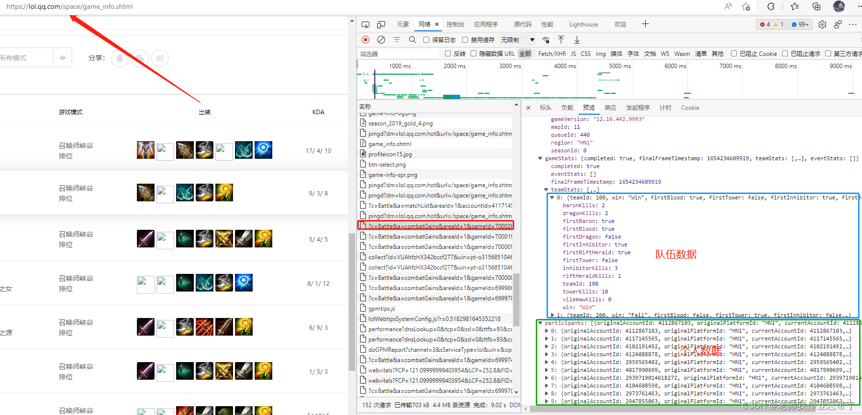
Although the process is a little troublesome, it is still simple , Those who are interested can climb by themselves ( notes : Domestic official website and opgg The returned information has its advantages and disadvantages , It is recommended to use opgg Crawling foreign service a player's record every event Little by little , For example, I used to teach with Dafei “hide on bush” For example , There are many games It is also the king of Korean clothes Quality Bureau .)
You can also use off the shelf :League of Legends Diamond Ranked Games (10 min) | Kaggle
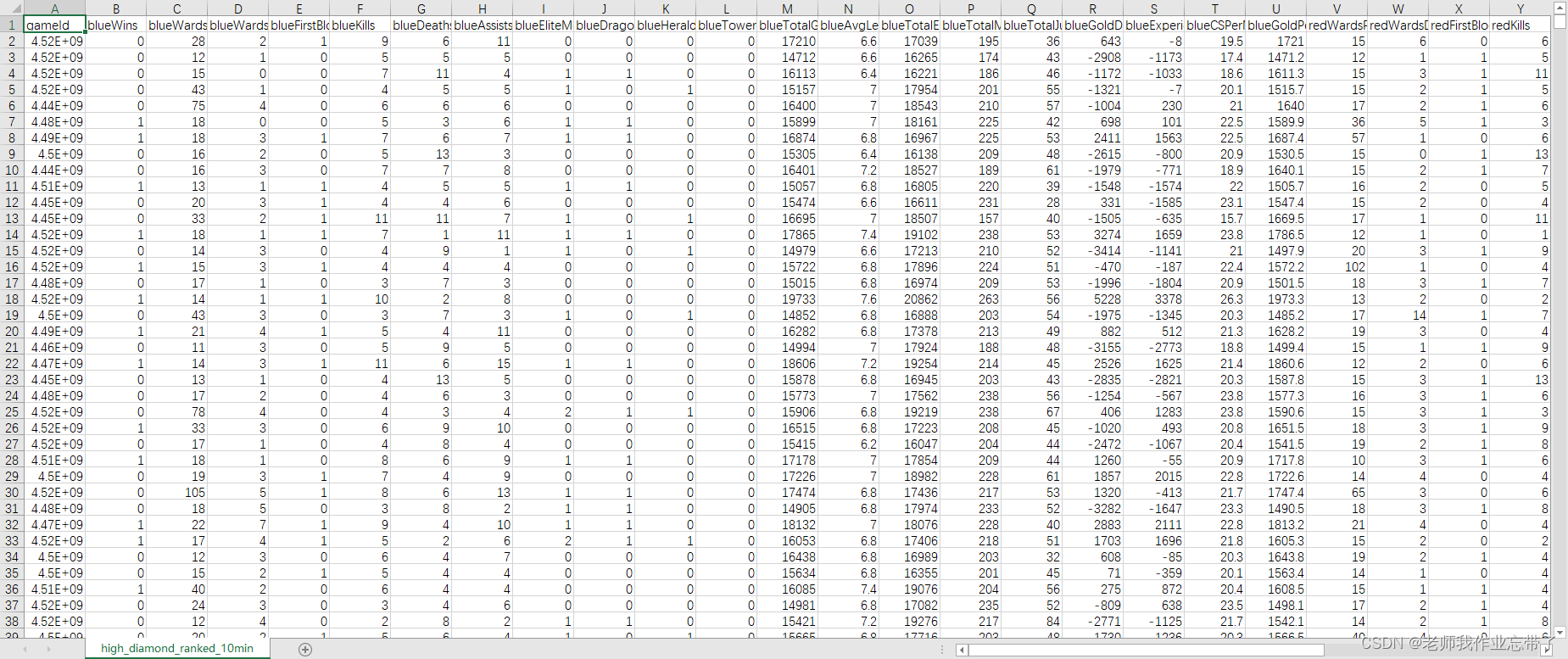
It includes 9879 Once the field drill reaches the master level Single double row Match up , The two sides are almost at the same level . Each data is the first 10 Minutes of match , Each team has 19 Features , The red and blue sides share 38 Features . These features include hero killing 、 Death , View 、 money 、 Experience 、 Level, etc .
The second step : Data processing
Import toolkit
import numpy as np
import pandas as pd
from collections import Counter
from sklearn.model_selection import train_test_split, cross_validate #  Partition dataset function
from sklearn.metrics import accuracy_score #  Accuracy function
RANDOM_SEED = 2020 #  Fix random seeds
Read in the data
csv_data = './data/high_diamond_ranked_10min.csv' #  Data path
data_df = pd.read_csv(csv_data, sep=',') #  Read in csv File for pandas Of DataFrame
data_df = data_df.drop(columns='gameId') #  Remove the match ID Column
An overview of the data
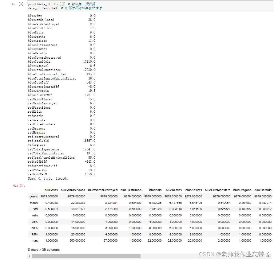
Have a general understanding of data distribution , For example, we can go through .iloc[0] Take the first row of data and output . It is not difficult to see that every feature exists float64 Floating point numbers , The game starts in blue 10 Minutes have a small advantage . At the same time, it can also be found that some feature columns are redundant , such as blueGoldDiff Indicates the gold coin advantage of the blue team ,redGoldDiff Indicates the advantage of Red Square Gold Coin , These two features are completely symmetrical and opposite to each other , wait .
such as blueKills The average number of heroes killed by the blue side in the first ten minutes is 6.14、 The variance of 2.93, The median is 6, In more than 50% of the matches, this feature is 4-8 Between , wait .
Addition and deletion features
Remove some miscellaneous information , And like the above-mentioned general blue side kill equals red side death , Or the number of blue and red square gold coins can be combined into economic difference , Or the Red Square happened 1 Blood is so blue that it doesn't happen ...
drop_features = ['blueGoldDiff', 'redGoldDiff',
                 'blueExperienceDiff', 'redExperienceDiff',
                 'blueCSPerMin', 'redCSPerMin',
                 'blueGoldPerMin', 'redGoldPerMin'] #  Feature columns that need to be rounded off
df = data_df.drop(columns=drop_features) #  Omit the characteristic column
info_names = [c[3:] for c in df.columns if c.startswith('red')] #  Take out the name of the feature to make the difference ( remove red Prefix )
for info in info_names: #  For each feature name
    df['br' + info] = df['blue' + info] - df['red' + info] #  Construct a new feature , Subtract the red feature from the blue feature , The prefix for br
#  among FirstBlood For the first kill, at most one team can get ,brFirstBlood=1 For blue ,0 For there is no ,-1 For red
df = df.drop(columns=['blueFirstBlood', 'redFirstBlood']) #  The original FirstBlood Deleting
After this step, the variable df From the original 38 Features -8( You don't need )+15( Red blue difference )-2( A blood ), There is still left 43 Eigenvalues , Plus whether the blue side wins , altogether 44 Column .
Feature discretization
Decision tree ID3 Algorithms are generally based on discrete features , There are many continuous numerical features in this example , For example, team gold coins . Directly applying each value of the algorithm as a value of the feature may cause serious over fitting , Therefore, it is necessary to discretize the features , That is, mapping a range of values into a value , For example, the age characteristics of users , take 0-10 Mapping to 0,11-18 Mapping to 1,19-25 Mapping to 2,25-30 Mapping to 3, And so on , Then, when building the decision tree, the mapped value is used to calculate the information gain .
DISCRETE_N = 10
discrete_df = df.copy()
for c in df.columns[1:]:
    if len(df[c].unique()) <= DISCRETE_N:
        continue
    else:
        discrete_df[c] = pd.qcut(df[c], DISCRETE_N, precision=0, labels=False, duplicates='drop')
notes : Some features themselves have few values , You can skip discretization .
Data set preparation
Take a random part, such as 20% Make a test set , The rest is a training set .sklearn Provides related tool functions train_test_split.sklearn The input and output of is generally numpy Of array matrix , You need to pandas Of DataFrame Take out as numpy Of array matrix .
all_y = discrete_df['blueWins'].values #  All tag data
feature_names = discrete_df.columns[1:] #  Names of all features
all_x = discrete_df[feature_names].values #  All original eigenvalues
#  Divide the training set and the test set
x_train, x_test, y_train, y_test = train_test_split(all_x, all_y, test_size=0.2, random_state=RANDOM_SEED)

# ((9879,), (9879, 43), (7903, 43), (1976, 43), (7903,), (1976,))
The third step : Implementation of decision tree model
Deleted and modified many times , It's a long way to go ~
#  Define decision tree classes
class DecisionTree(object):
    def __init__(self, classes, features,
                 max_depth=10, min_samples_split=10,
                 impurity_t='entropy'):
        '''
         Pass in some possible model parameters , It may not be used
        classes There are several types of model classification
        features Is the name of each feature , It is also convenient to query the total number of common features
        max_depth Represents the maximum depth when building the decision tree
        min_samples_split Indicates that when building the split node of the decision tree , If the number of samples arriving at this node is less than this value, it will not split
        impurity_t Indicates the calculated confounding ( Impure ) Calculation method of , for example entropy or gini
        '''
        self.classes = classes
        self.features = features
        self.max_depth = max_depth
        self.min_samples_split = min_samples_split
        self.impurity_t = impurity_t
        self.root = None  #  Define the root node , Empty when not training

    def impurity(self, data):
        '''
         Calculate the information gain under a certain feature
        :param data: ,numpy One dimensional array
        :return:  Promiscuity
        '''
        cnt = Counter(data)  #  Count the number of occurrences of each value
        probability_lst = [1.0 * cnt[i] / len(data) for i in cnt]
        if self.impurity_t == 'entropy':  #  If it is information entropy
            return -np.sum([p * np.log2(p) for p in probability_lst if p > 0]), cnt  #  Return entropy   And the number of data that may be used ( Convenient for future use )
        return 1 - np.sum([p * p for p in probability_lst]), cnt  #  Otherwise return to gini coefficient

    def gain(self, feature, label):
        '''
         Calculate the information gain under a certain feature
        :param feature:  The value of the feature ,numpy One dimensional array
        :param label:  Corresponding label ,numpy One dimensional array
        :return:  Information gain
        '''
        c_impurity, _ = self.impurity(label)  #  The promiscuous degree of labels without considering features

        #  Record the array subscript corresponding to each value of the feature
        f_index = {}
        for idx, v in enumerate(feature):
            if v not in f_index:
                f_index[v] = []
            f_index[v].append(idx)

        #  Calculate the impurity after splitting according to this feature , Weighted sum according to the number of each value of the feature
        f_impurity = 0
        for v in f_index:
            #  Take the corresponding array subscript according to the feature   Take out the corresponding tag list   Branches such as 1 How many positive and negative examples   Branch 2 Yes ...
            f_l = label[f_index[v]]
            f_impurity += self.impurity(f_l)[0] * len(f_l) / len(label)  #  At the end of the loop, we get the expectation of the hybrid degree of each branch

        gain = c_impurity - f_impurity  #  obtain gain

        #  Some features take many values , Natural impurity is high 、 High information gain , The model will favor features with many values, such as date , But it is likely to over fit
        #  Calculating the information gain rate can alleviate this problem
        splitInformation = self.impurity(feature)[0]  #  Calculate the impurity of this feature when it is label independent
        gainRatio = gain / splitInformation if splitInformation > 0 else gain  #  The divisor is not 0 Is the information gain rate
        return gainRatio, f_index  #  Return information gain rate , And the array subscript of each feature value ( Convenient for future use )

    def expand_node(self, feature, label, depth, skip_features=set()):
        '''
         Recursive function splits nodes
        :param feature: A two-dimensional numpy(n*m) Array , Each line represents a sample ,n That's ok , Yes m Features
        :param label: A one-dimensional numpy(n) Array , Indicates the classification label of each sample
        :param depth: The depth of the current node
        :param skip_features: Indicates the features that have been used in the current path
         At present ID3 Implementation of discrete features of the algorithm , Features that have been used on a path will no longer be used ( Other implementations may choose repetitive features )
        '''

        l_cnt = Counter(label)  #  Count the number of samples in each category
        if len(l_cnt) <= 1:  #  If there is only one category , No need to split , It's already a leaf node
            return label[0]  #  Just record the category
        if len(label) < self.min_samples_split or depth > self.max_depth:  #  If the minimum number of split samples or the maximum depth threshold is reached
            return l_cnt.most_common(1)[0][0]  #  Then only record the most categories in the current sample

        f_idx, max_gain, f_v_index = -1, -1, None  #  Prepare to pick split features
        for idx in range(len(self.features)):  #  Traverse all features
            if idx in skip_features:  #  If the current path has been used , Don't count
                continue
            f_gain, fv = self.gain(feature[:, idx], label)  #  Calculate the information gain of the feature ,fv Is the sample subscript of each value of the feature

            # if f_gain <= 0: #  If the information gain is not positive , Skip this feature
            #   continue
            if f_idx < 0 or f_gain > max_gain:  #  If a better split feature
                f_idx, max_gain, f_v_index = idx, f_gain, fv  #  Then record the characteristic

            # if f_idx < 0: #  If you don't find the right characteristics , That is, all features have no information gain
            #   return l_cnt.most_common(1)[0][0] #  Then only record the most categories in the current sample

        decision = {}  #  Use a dictionary to record the child nodes corresponding to each feature value ,key It's characteristic value ,value Is a child node
        skip_features = set([f_idx] + [f for f in skip_features])  #  The features to be skipped by child nodes include the currently selected features
        for v in f_v_index:  #  Traverse each value of the feature
            decision[v] = self.expand_node(feature[f_v_index[v], :], label[f_v_index[v]],  #  Take out the sample corresponding to the characteristic value
                                           depth=depth + 1, skip_features=skip_features)  #  depth +1, Recursive call node splitting
        #  Returns a tuple , There are three elements
        #  The first is the selected feature subscript , The second feature value and the corresponding child nodes ( Dictionaries ), The third is the category with the most samples reaching the current node
        return (f_idx, decision, l_cnt.most_common(1)[0][0])

    def traverse_node(self, node, feature):
        '''
         When predicting samples, traverse the nodes from the root node , Route according to characteristics .
        :param node:  Currently arriving node , for example self.root
        :param feature:  The length is m Of numpy One dimensional array
        '''
        assert len(self.features) == len(feature)  #  It is required that the number of features of the input sample is consistent with that of the model definition
        if type(node) is not tuple:  #  If a node is reached, it is a leaf node ( No longer split ), Then return the node category
            return node
        fv = feature[node[0]]  #  Otherwise, take out the corresponding eigenvalue of the node ,node[0] The subscript of the feature is recorded
        if fv in node[1]:  #  Find the child node according to the eigenvalue , Note that it is necessary to judge whether the samples arriving at the training node when it is split have the eigenvalue ( Branch )
            return self.traverse_node(node[1][fv], feature)  #  If there is , Then enter the child node and continue to traverse
        return node[-1]  #  without , Return to the category with the most samples reaching the current node during training

    def fit(self, feature, label):
        '''
         Training models
        :param feature:feature Is 2D numpy(n*m) Array , Each line represents a sample , Yes m Features
        :param label:label One dimensional numpy(n) Array , Indicates the classification label of each sample
        '''
        assert len(self.features) == len(feature[0])  #  The number of features of the input data should be the same as that of the model definition
        self.root = self.expand_node(feature, label, depth=1)  #  Split from the root node , Model record root node

    def predict(self, feature):
        '''
         forecast
        :param feature: Input feature It can be a one-dimensional numpy The array can also be a two-dimensional numpy Array
         If it's one dimension numpy(m) Array is a sample , contain m Features , Return a category value
         If it's two-dimensional numpy(n*m) Arrays represent n Samples , Each sample contains m Features , Return to one numpy One dimensional array
        '''
        assert len(feature.shape) == 1 or len(feature.shape) == 2  #  Can only be 1 Dimension or 2 dimension
        if len(feature.shape) == 1:  #  If it is a sample
            return self.traverse_node(self.root, feature)  #  Start routing from the root node
        return np.array([self.traverse_node(self.root, f) for f in feature])  #  If there are many samples

    def get_params(self, deep):  #  To be called sklearn Of cross_validate You need to implement this function to return all parameters
        return {'classes': self.classes, 'features': self.features,
                'max_depth': self.max_depth, 'min_samples_split': self.min_samples_split,
                'impurity_t': self.impurity_t}

    def set_params(self, **parameters):  #  To be called sklearn Of GridSearchCV You need to implement this function to set all parameters for the class
        for parameter, value in parameters.items():
            setattr(self, parameter, value)
        return self


#  Define decision tree model , Pass in algorithm parameters
DT = DecisionTree(classes=[0, 1], features=feature_names, max_depth=5, min_samples_split=10, impurity_t='gini')

DT.fit(x_train, y_train)  #  Train on the training set
p_test = DT.predict(x_test)  #  Predict on the test set , Obtain the predicted value
print(p_test)  #  Output predicted value
test_acc = accuracy_score(p_test, y_test)  #  Compare the test prediction value with the test set label to obtain the accuracy
print('accuracy: {:.4f}'.format(test_acc))  #  Output accuracy
[0 1 0 ... 0 1 1]
accuracy: 0.6964
The accuracy rate at this time is 0.6964, Let's tune the model .
Step four : Model tuning
Different calculation methods of hybrid degree on the test set 、 depth 、 Minimum split threshold for 50% cross validation .
%%time

best = None #  Record the best results
for impurity_t in ['entropy', 'gini']: #  Traverse the calculation method of impurity
    for max_depth in range(1, 6): #  Traverse the maximum tree depth
        for min_samples_split in [50, 100, 200, 500, 1000]: #  Traverse the threshold of the minimum number of samples for node splitting
            DT = DecisionTree(classes=[0,1], features=feature_names,  #  Define the decision tree
                              max_depth=max_depth, min_samples_split=min_samples_split, impurity_t=impurity_t)
            cv_result = cross_validate(DT, x_train, y_train, scoring=('accuracy'), cv=5) # 5 Crossover verification
            cv_acc = np.mean(cv_result['test_score']) # 5 Average accuracy
            current = (cv_acc, max_depth, min_samples_split, impurity_t) #  Record parameters and results
            if best is None or cv_acc > best[0]: #  If it is a better result than the current best
                best = current #  Record the best results
                print('better cv_accuracy: {:.4f}, max_depth={}, min_samples_split={}, impurity_t={}'.format(*best)) #  Output accuracy and parameters
            else:
                print('cv_accuracy: {:.4f}, max_depth={}, min_samples_split={}, impurity_t={}'.format(*current)) #  Output accuracy and parameters

DT = DecisionTree(classes=[0,1], features=feature_names, max_depth=best[1], min_samples_split=best[2], impurity_t=best[3])  #  Take the best parameters
DT.fit(x_train, y_train) #  Train on the training set
p_test = DT.predict(x_test) #  Predict on the test set , Obtain the predicted value
print(p_test) #  Output predicted value
test_acc = accuracy_score(p_test, y_test) #  Compare the test prediction value with the test set label to obtain the accuracy
print('accuracy: {:.4f}'.format(test_acc)) #  Output accuracy
better cv_accuracy: 0.7257, max_depth=1, min_samples_split=50, impurity_t=entropy cv_accuracy: 0.7257, max_depth=1, min_samples_split=100, impurity_t=entropy cv_accuracy: 0.7257, max_depth=1, min_samples_split=200, impurity_t=entropy cv_accuracy: 0.7257, max_depth=1, min_samples_split=500, impurity_t=entropy cv_accuracy: 0.7257, max_depth=1, min_samples_split=1000, impurity_t=entropy cv_accuracy: 0.7254, max_depth=2, min_samples_split=50, impurity_t=entropy cv_accuracy: 0.7254, max_depth=2, min_samples_split=100, impurity_t=entropy cv_accuracy: 0.7254, max_depth=2, min_samples_split=200, impurity_t=entropy cv_accuracy: 0.7254, max_depth=2, min_samples_split=500, impurity_t=entropy cv_accuracy: 0.7257, max_depth=2, min_samples_split=1000, impurity_t=entropy better cv_accuracy: 0.7267, max_depth=3, min_samples_split=50, impurity_t=entropy better cv_accuracy: 0.7272, max_depth=3, min_samples_split=100, impurity_t=entropy better cv_accuracy: 0.7281, max_depth=3, min_samples_split=200, impurity_t=entropy better cv_accuracy: 0.7286, max_depth=3, min_samples_split=500, impurity_t=entropy cv_accuracy: 0.7257, max_depth=3, min_samples_split=1000, impurity_t=entropy cv_accuracy: 0.7237, max_depth=4, min_samples_split=50, impurity_t=entropy cv_accuracy: 0.7252, max_depth=4, min_samples_split=100, impurity_t=entropy cv_accuracy: 0.7285, max_depth=4, min_samples_split=200, impurity_t=entropy better cv_accuracy: 0.7290, max_depth=4, min_samples_split=500, impurity_t=entropy cv_accuracy: 0.7257, max_depth=4, min_samples_split=1000, impurity_t=entropy cv_accuracy: 0.7149, max_depth=5, min_samples_split=50, impurity_t=entropy cv_accuracy: 0.7210, max_depth=5, min_samples_split=100, impurity_t=entropy cv_accuracy: 0.7254, max_depth=5, min_samples_split=200, impurity_t=entropy cv_accuracy: 0.7290, max_depth=5, min_samples_split=500, impurity_t=entropy cv_accuracy: 0.7257, max_depth=5, min_samples_split=1000, impurity_t=entropy cv_accuracy: 0.7257, max_depth=1, min_samples_split=50, impurity_t=gini cv_accuracy: 0.7257, max_depth=1, min_samples_split=100, impurity_t=gini cv_accuracy: 0.7257, max_depth=1, min_samples_split=200, impurity_t=gini cv_accuracy: 0.7257, max_depth=1, min_samples_split=500, impurity_t=gini cv_accuracy: 0.7257, max_depth=1, min_samples_split=1000, impurity_t=gini cv_accuracy: 0.7255, max_depth=2, min_samples_split=50, impurity_t=gini cv_accuracy: 0.7255, max_depth=2, min_samples_split=100, impurity_t=gini cv_accuracy: 0.7255, max_depth=2, min_samples_split=200, impurity_t=gini cv_accuracy: 0.7255, max_depth=2, min_samples_split=500, impurity_t=gini cv_accuracy: 0.7257, max_depth=2, min_samples_split=1000, impurity_t=gini cv_accuracy: 0.7218, max_depth=3, min_samples_split=50, impurity_t=gini cv_accuracy: 0.7235, max_depth=3, min_samples_split=100, impurity_t=gini cv_accuracy: 0.7250, max_depth=3, min_samples_split=200, impurity_t=gini cv_accuracy: 0.7257, max_depth=3, min_samples_split=500, impurity_t=gini cv_accuracy: 0.7257, max_depth=3, min_samples_split=1000, impurity_t=gini cv_accuracy: 0.7174, max_depth=4, min_samples_split=50, impurity_t=gini cv_accuracy: 0.7248, max_depth=4, min_samples_split=100, impurity_t=gini cv_accuracy: 0.7261, max_depth=4, min_samples_split=200, impurity_t=gini cv_accuracy: 0.7259, max_depth=4, min_samples_split=500, impurity_t=gini cv_accuracy: 0.7257, max_depth=4, min_samples_split=1000, impurity_t=gini cv_accuracy: 0.7076, max_depth=5, min_samples_split=50, impurity_t=gini cv_accuracy: 0.7185, max_depth=5, min_samples_split=100, impurity_t=gini cv_accuracy: 0.7207, max_depth=5, min_samples_split=200, impurity_t=gini cv_accuracy: 0.7259, max_depth=5, min_samples_split=500, impurity_t=gini cv_accuracy: 0.7257, max_depth=5, min_samples_split=1000, impurity_t=gini
Use max_depth=4, min_samples_split=500, impurity_t=entropy Training on a training set , And predict on the test set , Compare the test prediction value with the test set label to obtain the accuracy : Obviously improved .
[0 1 0 ... 0 1 1]
accuracy: 0.7171
Wall time: 1min 19s
You can also call sklearn Of GridSearchCV Automatic and multithreaded search parameters , Similar to the above process .
%%time

parameters = {'impurity_t':['entropy', 'gini'],
              'max_depth': range(1, 6),
              'min_samples_split': [50, 100, 200, 500, 1000]} #  Define the parameters that need to be traversed
DT = DecisionTree(classes=[0,1], features=feature_names) #  Define the decision tree , No parameters can be passed , from GridSearchCV Incoming build
grid_search = GridSearchCV(DT, parameters, scoring='accuracy', cv=5, verbose=100, n_jobs=4) #  Pass in the model and the parameters to traverse
grid_search.fit(x_train, y_train) #  Search for parameters on all data
print(grid_search.best_score_, grid_search.best_params_) #  Output the best indicators and parameters

DT = DecisionTree(classes=[0,1], features=feature_names, **grid_search.best_params_)  #  Take the best parameters
DT.fit(x_train, y_train) #  Train on the training set
p_test = DT.predict(x_test) #  Predict on the test set , Obtain the predicted value
print(p_test) #  Output predicted value
test_acc = accuracy_score(p_test, y_test) #  Compare the test prediction value with the test set label to obtain the accuracy
print('accuracy: {:.4f}'.format(test_acc)) #  Output accuracy
Fitting 5 folds for each of 50 candidates, totalling 250 fits
0.7289642831407777 {'impurity_t': 'entropy', 'max_depth': 4, 'min_samples_split': 500}
[0 1 0 ... 0 1 1]
accuracy: 0.7171
Wall time: 24.6 sView the characteristics of the node
best_dt = grid_search.best_estimator_ #  Take out the best model
print('root', best_dt.features[best_dt.root[0]]) #  Output root node characteristics
root brTotalGold
Visible before 10 Minutes can affect the winning rate most The economic difference between red and blue
for fv in best_dt.root[1]: #  Traverse each characteristic value of the root node
    print(fv, '->', best_dt.features[best_dt.root[1][fv][0]], '-> ...') #  Output the next level of features
9 -> redDragons -> ... 1 -> blueTowersDestroyed -> ... 3 -> redEliteMonsters -> ... 5 -> redTowersDestroyed -> ... 2 -> blueTowersDestroyed -> ... 4 -> brTowersDestroyed -> ... 7 -> redEliteMonsters -> ... 8 -> brTowersDestroyed -> ... 0 -> brKills -> ... 6 -> brTowersDestroyed -> ...
The root node corresponds to the value 0-9( We discretized the gold coins before ) Corresponding to the characteristics of the next layer ...
ps: This actually comes from what we define expand_node Function return value ,
return (f_idx, decision, l_cnt.most_common(1)[0][0]) ,
The first is the selected feature subscript , The second feature value and the corresponding child nodes ( Dictionaries ), The third is the category with the most samples reaching the current node .
Its shape / It turns out to be :
(38,
 {9: (20,
   {0: (23, {1: 1, 2: 1, 4: 1, 0: 1, 3: 1, 5: 1, 6: 1, 7: 1, 8: 1}, 1), 1: 1},
   1),
  1: (8, {0: (7, {0: (20, {1: 0, 0: 0}, 0), 1: 0}, 0), 1: 0}, 0),
  3: (19, {0: 0, 1: 0, 2: 0}, 0),
  5: (22, {0: (19, {0: 1, 2: 0, 1: 0}, 1), 1: 1, 2: 1}, 1),
  2: (8, {0: (22, {0: (6, {0: 0, 1: 0}, 0), 1: 0, 2: 1}, 0), 1: 1}, 0),
  4: (37, {0: (8, {0: (5, {0: 0, 1: 0, 2: 1}, 0), 1: 1}, 0), -1: 0, 1: 0}, 0),
  7: (19, {1: 1, 0: 1, 2: 1}, 1),
  8: (37, {0: (8, {0: (6, {0: 1, 1: 1}, 1), 1: 1}, 1), 1: 1, 2: 1}, 1),
  0: (31, {0: (5, {0: 0, 1: 0, 2: 0}, 0), 1: 0, 2: 0, 4: 0, 3: 0}, 0),
  6: (37, {0: (8, {0: (6, {1: 1, 0: 1}, 1), 1: 1}, 1), 1: 0, 2: 1, -1: 0}, 1)},
 0)
边栏推荐
- Reptile practice (VIII): reptile expression pack
- The weight of the product page of the second level classification is low. What if it is not included?
- Kubernetes Static Pod (静态Pod)
- Letcode43: string multiplication
- Qt不同类之间建立信号槽,并传递参数
- 什么是负载均衡?DNS如何实现负载均衡?
- DNS series (I): why does the updated DNS record not take effect?
- Where is the big data open source project, one-stop fully automated full life cycle operation and maintenance steward Chengying (background)?
- NTT template for Tourism
- LeetCode刷题
猜你喜欢
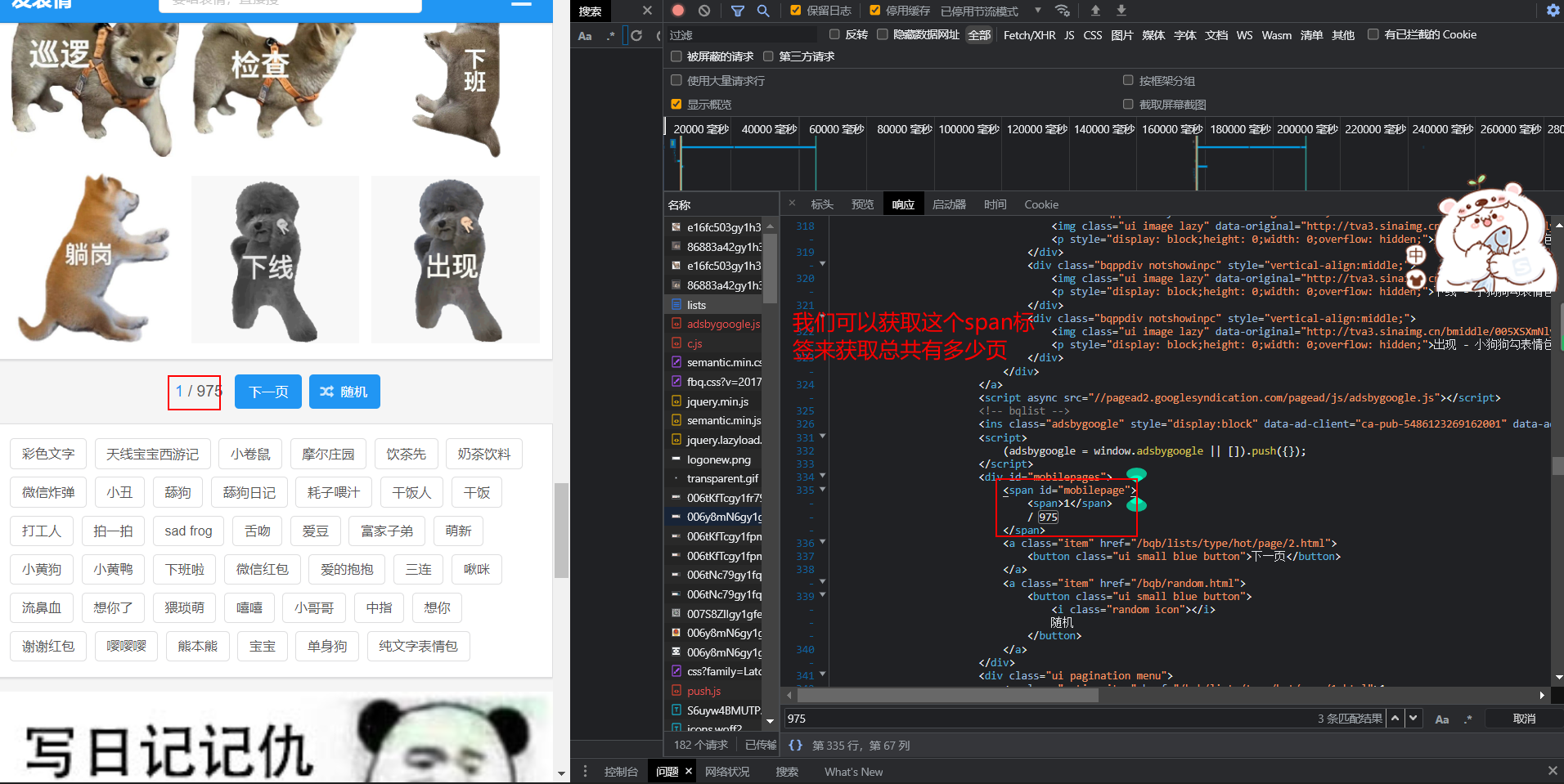
Reptile practice (VIII): reptile expression pack
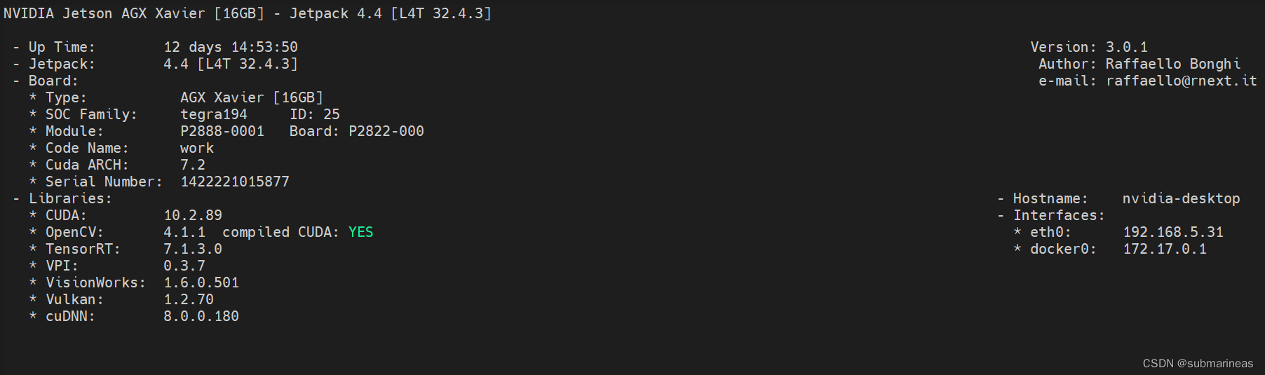
NVIDIA Jetson test installation yolox process record

QT adds resource files, adds icons for qaction, establishes signal slot functions, and implements
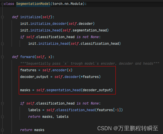
语义分割模型库segmentation_models_pytorch的详细使用介绍
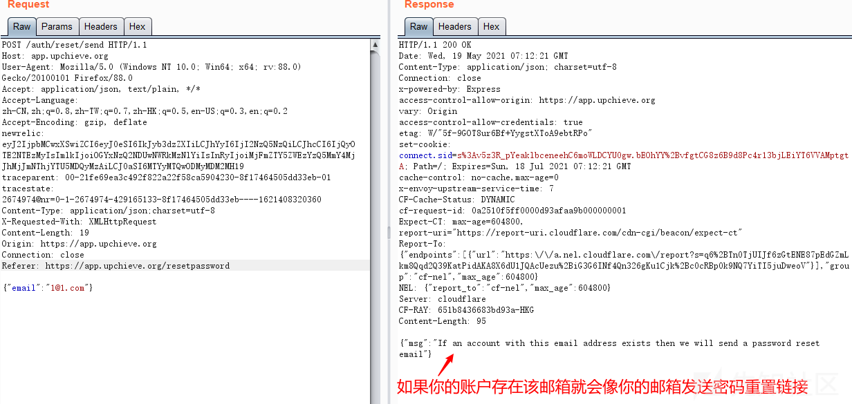
Password recovery vulnerability of foreign public testing

What has happened from server to cloud hosting?

What does interface testing test?
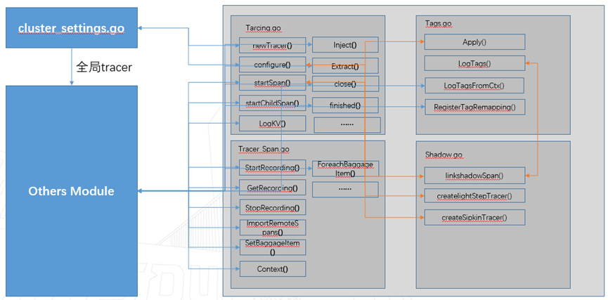
Langchao Yunxi distributed database tracing (II) -- source code analysis
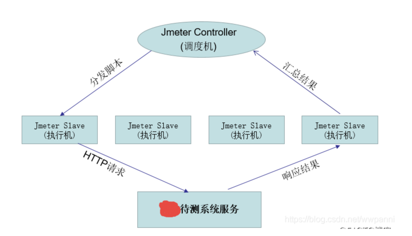
Jemter distributed
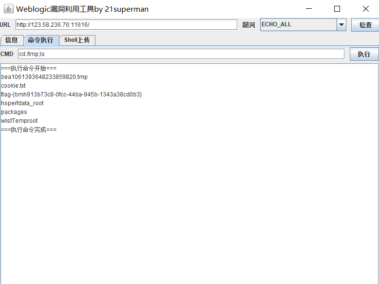
Fofa attack and defense challenge record
随机推荐
How does the markdown editor of CSDN input mathematical formulas--- Latex syntax summary
【愚公系列】2022年7月 Go教学课程 006-自动推导类型和输入输出
C# 泛型及性能比较
Installation and configuration of sublime Text3
赞!idea 如何单窗口打开多个项目?
[note] common combined filter circuit
Invalid V-for traversal element style
Introduction to paddle - using lenet to realize image classification method I in MNIST
玩轉Sonar
Summary of weidongshan phase II course content
[go record] start go language from scratch -- make an oscilloscope with go language (I) go language foundation
8道经典C语言指针笔试题解析
CVE-2022-28346:Django SQL注入漏洞
C # generics and performance comparison
攻防演练中沙盘推演的4个阶段
They gathered at the 2022 ecug con just for "China's technological power"
Basic types of 100 questions for basic grammar of Niuke
股票开户免费办理佣金最低的券商,手机上开户安全吗
【愚公系列】2022年7月 Go教学课程 006-自动推导类型和输入输出
Service Mesh介绍,Istio概述