Credit card fraud detection based on machine learning

One 、 Credit card fraud detection based on machine learning

1.1 Preface

1. Data sources ：Kaggle Credit card fraud detection data set https://www.kaggle.com/datasets/mlg-ulb/creditcardfraud?resource=download;
2. In this paper XGBoost、 Random forests 、KNN、 Logical regression 、SVM And decision tree to solve the problem of credit card fraud detection ;

1.2 case analysis

1.2.1 Import the required modules to python Environmental Science

# 1、 Import the required modules to  python  Environment 
import pandas as pd
import numpy as np
import matplotlib.pyplot as plt
from termcolor import colored as cl
import itertools
from sklearn.preprocessing import StandardScaler
from sklearn.model_selection import train_test_split
from sklearn.tree import DecisionTreeClassifier
from sklearn.neighbors import KNeighborsClassifier
from sklearn.linear_model import LogisticRegression
from sklearn.svm import SVC
from sklearn.ensemble import RandomForestClassifier
from xgboost import XGBClassifier
from sklearn.metrics import confusion_matrix, accuracy_score, f1_score

1.2.2 Reading data , Delete useless Time Column

• About data ： The data we are going to use is Kaggle Credit card fraud detection data set . It contains V1 To V28, yes PCA The main ingredients obtained , And ignore time features that are not useful for building models .
• The remaining features are... Including the total transaction amount " amount of money " Characteristics and information on whether the transaction is a fraud case " Category " features , Category 0 Identification fraud , Category 1 Is normal .

df = pd.read_csv(r'../creditcard.csv')
print("Data's columns contain:\n", df.columns)
print("Data shape:\n", df.shape)
df.drop('Time', axis=1, inplace=True)
pd.set_option('display.max_columns', df.shape[1])
print(df.head())
''' Data's columns contain: Index(['Time', 'V1', 'V2', 'V3', 'V4', 'V5', 'V6', 'V7', 'V8', 'V9', 'V10', 'V11', 'V12', 'V13', 'V14', 'V15', 'V16', 'V17', 'V18', 'V19', 'V20', 'V21', 'V22', 'V23', 'V24', 'V25', 'V26', 'V27', 'V28', 'Amount', 'Class'], dtype='object') Data shape: (284807, 31) V1 V2 V3 V4 V5 V6 V7 \ 0 -1.359807 -0.072781 2.536347 1.378155 -0.338321 0.462388 0.239599 1 1.191857 0.266151 0.166480 0.448154 0.060018 -0.082361 -0.078803 2 -1.358354 -1.340163 1.773209 0.379780 -0.503198 1.800499 0.791461 3 -0.966272 -0.185226 1.792993 -0.863291 -0.010309 1.247203 0.237609 4 -1.158233 0.877737 1.548718 0.403034 -0.407193 0.095921 0.592941 V8 V9 V10 V11 V12 V13 V14 \ 0 0.098698 0.363787 0.090794 -0.551600 -0.617801 -0.991390 -0.311169 1 0.085102 -0.255425 -0.166974 1.612727 1.065235 0.489095 -0.143772 2 0.247676 -1.514654 0.207643 0.624501 0.066084 0.717293 -0.165946 3 0.377436 -1.387024 -0.054952 -0.226487 0.178228 0.507757 -0.287924 4 -0.270533 0.817739 0.753074 -0.822843 0.538196 1.345852 -1.119670 V15 V16 V17 V18 V19 V20 V21 \ 0 1.468177 -0.470401 0.207971 0.025791 0.403993 0.251412 -0.018307 1 0.635558 0.463917 -0.114805 -0.183361 -0.145783 -0.069083 -0.225775 2 2.345865 -2.890083 1.109969 -0.121359 -2.261857 0.524980 0.247998 3 -0.631418 -1.059647 -0.684093 1.965775 -1.232622 -0.208038 -0.108300 4 0.175121 -0.451449 -0.237033 -0.038195 0.803487 0.408542 -0.009431 V22 V23 V24 V25 V26 V27 V28 \ 0 0.277838 -0.110474 0.066928 0.128539 -0.189115 0.133558 -0.021053 1 -0.638672 0.101288 -0.339846 0.167170 0.125895 -0.008983 0.014724 2 0.771679 0.909412 -0.689281 -0.327642 -0.139097 -0.055353 -0.059752 3 0.005274 -0.190321 -1.175575 0.647376 -0.221929 0.062723 0.061458 4 0.798278 -0.137458 0.141267 -0.206010 0.502292 0.219422 0.215153 Amount Class 0 149.62 0 1 2.69 0 2 378.66 0 3 123.50 0 4 69.99 0 '''

1.2.3 Exploratory data analysis and data preprocessing

cases = len(df)
nonfraud_cases = df[df.Class == 0]  #  Non fraud 
fraud_cases = df[df.Class == 1]  #  cheat 
fraud_percentage = round(len(nonfraud_cases) / cases * 100, 2)
print(cl('CASE COUNT', attrs=['bold']))
print(cl('-' * 40, attrs=['bold']))
print(cl('Total number of cases are {}'.format(cases), attrs=['bold']))
print(cl('Number of Non-fraud cases are {}'.format(len(nonfraud_cases)), attrs=['bold']))
print(cl('Number of fraud cases are {}'.format(len(fraud_cases)), attrs=['bold']))
print(cl('Percentage of fraud cases is {}%'.format(fraud_percentage), attrs=['bold']))
print(cl('-' * 40, attrs=['bold']))
print(cl('CASE AMOUNT STATISTICS', attrs=['bold']))
print(cl('-' * 40, attrs=['bold']))
print(cl('NON-FRAUD CASE AMOUNT STATS', attrs=['bold']))
print(nonfraud_cases.Amount.describe())
print(cl('-' * 40, attrs=['bold']))
print(cl('FRAUD CASE AMOUNT STATS', attrs=['bold']))
print(fraud_cases.Amount.describe())
print(cl('-' * 40, attrs=['bold']))
#  By looking at ,‘Amount’ The amount changes greatly , It needs to be standardized 
sc = StandardScaler()
amount = df.Amount.values
df.Amount = sc.fit_transform(amount.reshape(-1, 1))
print(cl(df.Amount.head(10), attrs=['bold']))
#  Feature selection and dataset splitting 
x = df.drop('Class', axis=1).values
y = df.Class.values
x_train, x_test, y_train, y_test = train_test_split(x, y, test_size=0.2, random_state=0)
''' CASE COUNT ---------------------------------------- Total number of cases are 284807 Number of Non-fraud cases are 284315 Number of fraud cases are 492 Percentage of fraud cases is 99.83% ---------------------------------------- CASE AMOUNT STATISTICS ---------------------------------------- NON-FRAUD CASE AMOUNT STATS count 284315.000000 mean 88.291022 std 250.105092 min 0.000000 25% 5.650000 50% 22.000000 75% 77.050000 max 25691.160000 Name: Amount, dtype: float64 ---------------------------------------- FRAUD CASE AMOUNT STATS count 492.000000 mean 122.211321 std 256.683288 min 0.000000 25% 1.000000 50% 9.250000 75% 105.890000 max 2125.870000 Name: Amount, dtype: float64 ---------------------------------------- 0 0.244964 1 -0.342475 2 1.160686 3 0.140534 4 -0.073403 5 -0.338556 6 -0.333279 7 -0.190107 8 0.019392 9 -0.338516 Name: Amount, dtype: float64'''

1.2.4 Build six classification models

1. Decision Tree

tree_model = DecisionTreeClassifier(max_depth=4, criterion='entropy').fit(x_train, y_train)
tree_yhat = tree_model.predict(x_test)

2. K-Nearest Neighbors

knn_model = KNeighborsClassifier(n_neighbors=5).fit(x_train, y_train)
knn_yhat = knn_model.predict(x_test)

3. Logistic Regression

lr_model = LogisticRegression().fit(x_train, y_train)
lr_yhat = lr_model.predict(x_test)

4. SVM

svm_model = SVC().fit(x_train, y_train)
svm_yhat = svm_model.predict(x_test)

5. Random Forest Tree

rf_model = RandomForestClassifier(max_depth=4).fit(x_train, y_train)
rf_yhat = rf_model.predict(x_test)

6. XGBoost

xgb_model = XGBClassifier(max_depth=4).fit(x_train, y_train)
xgb_yhat = xgb_model.predict(x_test)

1.2.5 Use evaluation indicators to evaluate the classification model created

1. Accuracy rate

print(cl('-' * 40, attrs=['bold']))
print(cl('ACCURACY SCORE', attrs=['bold']))
print(cl('Accuracy score of the Decision Tree model is {}'.format(round(accuracy_score(y_test, tree_yhat), 4)),
         attrs=['bold']))
print(cl('Accuracy score of the knn model is {}'.format(round(accuracy_score(y_test, knn_yhat), 4)), attrs=['bold']))
print(cl('Accuracy score of the Logistic Regression model is {}'.format(round(accuracy_score(y_test, lr_yhat), 4)),
         attrs=['bold']))
print(cl('Accuracy score of the SVM model is {}'.format(round(accuracy_score(y_test, svm_yhat), 4)), attrs=['bold']))
print(cl('Accuracy score of the Random Forest model is {}'.format(round(accuracy_score(y_test, rf_yhat), 4)),
         attrs=['bold']))
print(
    cl('Accuracy score of the XGBoost model is {}'.format(round(accuracy_score(y_test, xgb_yhat), 4)), attrs=['bold']))
''' ACCURACY SCORE Accuracy score of the Decision Tree model is 0.9994 Accuracy score of the knn model is 0.9995 Accuracy score of the Logistic Regression model is 0.9992 Accuracy score of the SVM model is 0.9993 Accuracy score of the Random Forest model is 0.9993 Accuracy score of the XGBoost model is 0.9995 '''

2. F1 value

print(cl('-' * 40, attrs=['bold']))
print(cl('F1 SCORE', attrs=['bold']))
print(cl('F1 score of the Decision Tree model is {}'.format(round(f1_score(y_test, tree_yhat), 4)), attrs=['bold']))
print(cl('F1 score of the knn model is {}'.format(round(f1_score(y_test, knn_yhat), 4)), attrs=['bold']))
print(cl('F1 score of the Logistic Regression model is {}'.format(round(f1_score(y_test, lr_yhat), 4)), attrs=['bold']))
print(cl('F1 score of the SVM model is {}'.format(round(f1_score(y_test, svm_yhat), 4)), attrs=['bold']))
print(cl('F1 score of the Random Forest model is {}'.format(round(f1_score(y_test, rf_yhat), 4)), attrs=['bold']))
print(cl('F1 score of the XGBoost model is {}'.format(round(f1_score(y_test, xgb_yhat), 4)), attrs=['bold']))
''' F1 SCORE F1 score of the Decision Tree model is 0.8105 F1 score of the knn model is 0.8571 F1 score of the Logistic Regression model is 0.7356 F1 score of the SVM model is 0.7771 F1 score of the Random Forest model is 0.7657 F1 score of the XGBoost model is 0.8449 '''

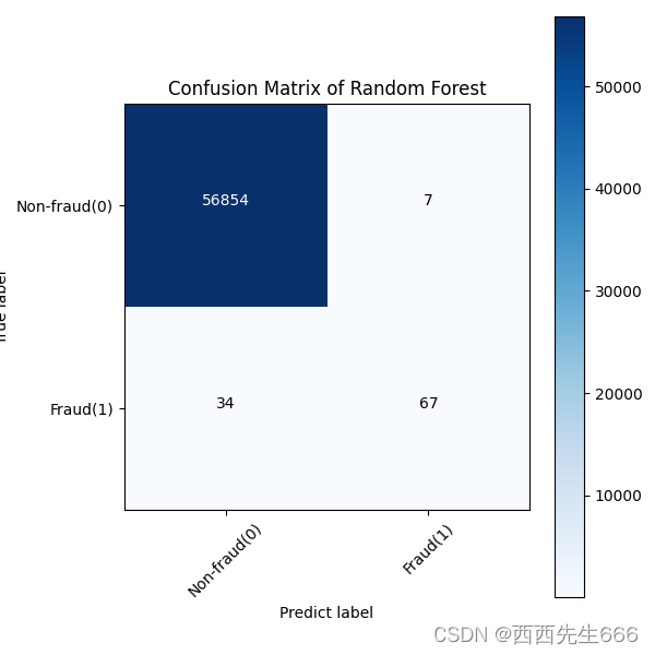
3. Confusion matrix

def plot_confusion_matrix(cm, classes, title, cmap=plt.cm.Blues):
    title = 'Confusion Matrix of {}'.format(title)
    plt.imshow(cm, cmap=cmap)
    plt.title(title)
    plt.colorbar()
    marks = np.arange(len(classes))
    plt.xticks(marks, classes, rotation=45)
    plt.yticks(marks, classes)
    thresh = cm.max() / 2
    for i, j in itertools.product(range(cm.shape[0]), range(cm.shape[1])):  #  The cartesian product 
        plt.text(j, i, format(cm[i, j], 'd'), horizontalalignment='center',
                 color='white' if cm[i, j] > thresh else 'black')
        """  Set text description  plt.text(x,y,string,fontsize=15,verticalalignment="top",horizontalalignment="right")  Parameters ： x,y: Represents the value on the coordinate value  string: To indicate caption  fontsize: Represents the font size  verticalalignment： Vertical alignment  , Parameters ：[ ‘center’ | ‘top’ | ‘bottom’ | ‘baseline’ ] horizontalalignment： Horizontal alignment  , Parameters ：[ ‘center’ | ‘right’ | ‘left’ ] """
    plt.tight_layout()
    plt.ylabel('True label')
    plt.xlabel('Predict label')

#  Calculating the confusion matrix 
tree_matrix = confusion_matrix(y_test, tree_yhat, labels=[0, 1])
knn_matrix = confusion_matrix(y_test, knn_yhat, labels=[0, 1])
lr_matrix = confusion_matrix(y_test, lr_yhat, labels=[0, 1])
svm_matrix = confusion_matrix(y_test, svm_yhat, labels=[0, 1])
rf_matrix = confusion_matrix(y_test, rf_yhat, labels=[0, 1])
xgb_matrix = confusion_matrix(y_test, xgb_yhat, labels=[0, 1])
#  adopt rc The configuration file is used to define various default properties of the graph 
plt.rcParams['figure.figsize'] = (6, 6)
classes = ['Non-fraud(0)', 'Fraud(1)']

tree_cm_plot = plot_confusion_matrix(tree_matrix,classes =classes, title='Decision Tree')
plt.savefig('tree_cm_plot.png')
plt.show()

The abscissa in the figure is predict label, The ordinate is true label;

knn_cm_plot = plot_confusion_matrix(knn_matrix,classes =classes, title='KNN')
plt.savefig('knn_cm_plot.png')
plt.show()

lr_cm_plot = plot_confusion_matrix(lr_matrix,classes =classes, title='Logistic Regression')
plt.savefig('lr_cm_plot.png')
plt.show()

svm_cm_plot = plot_confusion_matrix(svm_matrix,classes =classes, title='SVM')
plt.savefig('svm_cm_plot.png')
plt.show()

rf_cm_plot = plot_confusion_matrix(rf_matrix,classes =classes, title='Random Forest')
plt.savefig('rf_cm_plot.png')
plt.show()

xgb_cm_plot = plot_confusion_matrix(xgb_matrix,classes =classes, title='XGBoost')
plt.savefig('xgb_cm_plot.png')
plt.show()