当前位置:网站首页>Complete DNN deep neural network CNN training with tensorflow to complete image recognition cases
Complete DNN deep neural network CNN training with tensorflow to complete image recognition cases
2022-07-03 13:36:00 【Haibao 7】
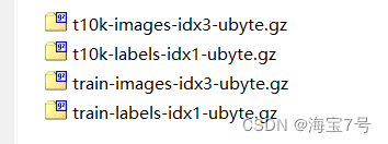
In deep learning , One of the more successful applications than traditional machine learning is image recognition . We use widely used MNIST Handwritten digital image data set .
Data set official website :
http://yann.lecun.com/exdb/mnist/
Use tensorflow complete DNN Deep neural network CNN Train to complete handwritten picture recognition
MNIST_data_bak Under the document Load source

The introduction and explanation in the program are very clear .
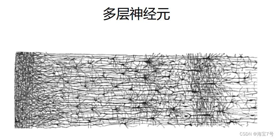
Talk with pictures , Self understanding >


Backpropagation
Back propagation , Gradient descent is used reverse-mode autodiff
• Forward propagation , Namely make predictions, Then calculate the output error , however
Then calculate the contribution of each neuron node to the error
• To seek contribution is to seek gradient according to the error of forward propagation
• Then adjust the original weight according to the contribution
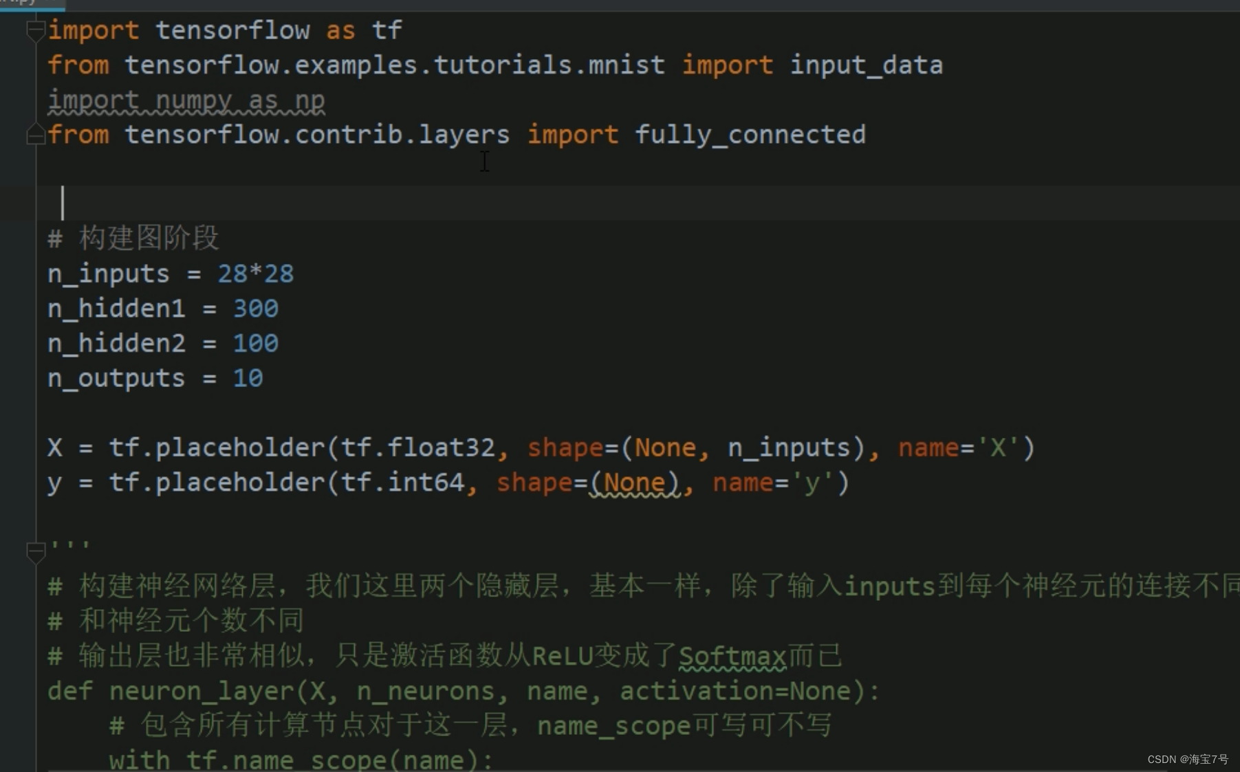
The code is as follows :
import tensorflow as tf
from tensorflow.examples.tutorials.mnist import input_data
import numpy as np
from tensorflow.contrib.layers import fully_connected
# The build diagram phase
n_inputs = 28*28
n_hidden1 = 300
n_hidden2 = 100
n_outputs = 10
X = tf.placeholder(tf.float32, shape=(None, n_inputs), name='X')
y = tf.placeholder(tf.int64, shape=(None), name='y')
# Build a neural network layer , We have two hidden layers here , Is essentially the same , In addition to the input inputs The connections to each neuron are different
# It's different from the number of neurons
# The output layer is also very similar , Just activate the function from ReLU Turned into Softmax nothing more
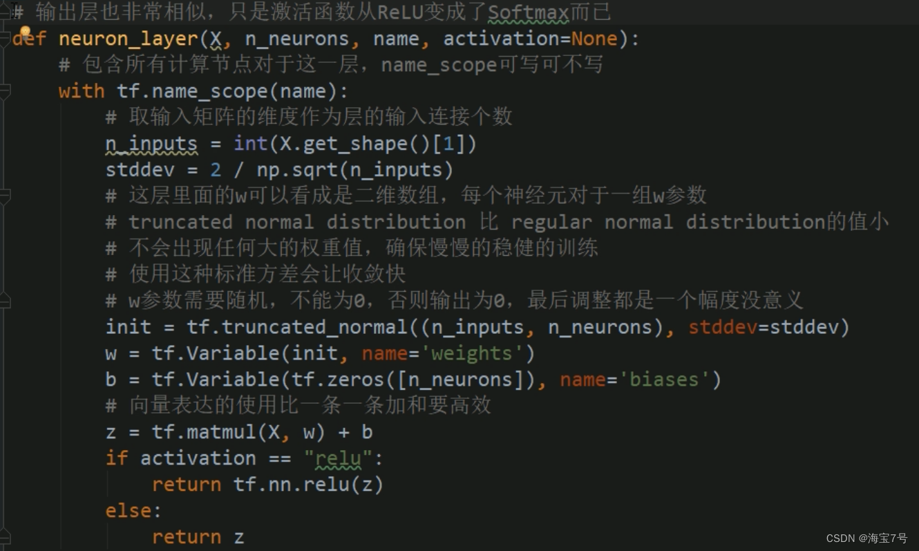
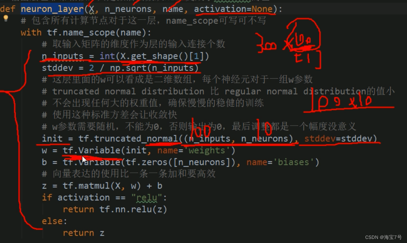
def neuron_layer(X, n_neurons, name, activation=None):
# Including all computing nodes for this layer ,name_scope Write but not write
with tf.name_scope(name):
# Take the dimension of the input matrix as the number of input connections of the layer
n_inputs = int(X.get_shape()[1])
stddev = 2 / np.sqrt(n_inputs)
# Inside this layer w Think of it as a two-dimensional array , Each neuron for a group of w Parameters
# truncated normal distribution Than regular normal distribution The value of is small
# There won't be any large weight values , Make sure you train slowly and steadily
# Using this standard variance will make the convergence faster
# w Parameters need to be random , Not for 0, Otherwise, the output is 0, Finally, the adjustment is not meaningful
init = tf.truncated_normal((n_inputs, n_neurons), stddev=stddev)
w = tf.Variable(init, name='weights')
b = tf.Variable(tf.zeros([n_neurons]), name='biases')
# The use of vector representations is more efficient than adding one by one
z = tf.matmul(X, w) + b
if activation == "relu":
return tf.nn.relu(z)
else:
return z
with tf.name_scope("dnn"):
hidden1 = neuron_layer(X, n_hidden1, "hidden1", activation="relu")
hidden2 = neuron_layer(hidden1, n_hidden2, "hidden2", activation="relu")
# Enter into softmax Previous results
logits = neuron_layer(hidden2, n_outputs, "outputs")
# with tf.name_scope("dnn"):
# # tensorflow Using this function helps us use the appropriate initialization w and b The strategy of , By default ReLU Activation function
# hidden1 = fully_connected(X, n_hidden1, scope="hidden1")
# hidden2 = fully_connected(hidden1, n_hidden2, scope="hidden2")
# logits = fully_connected(hidden2, n_outputs, scope="outputs", activation_fn=None)
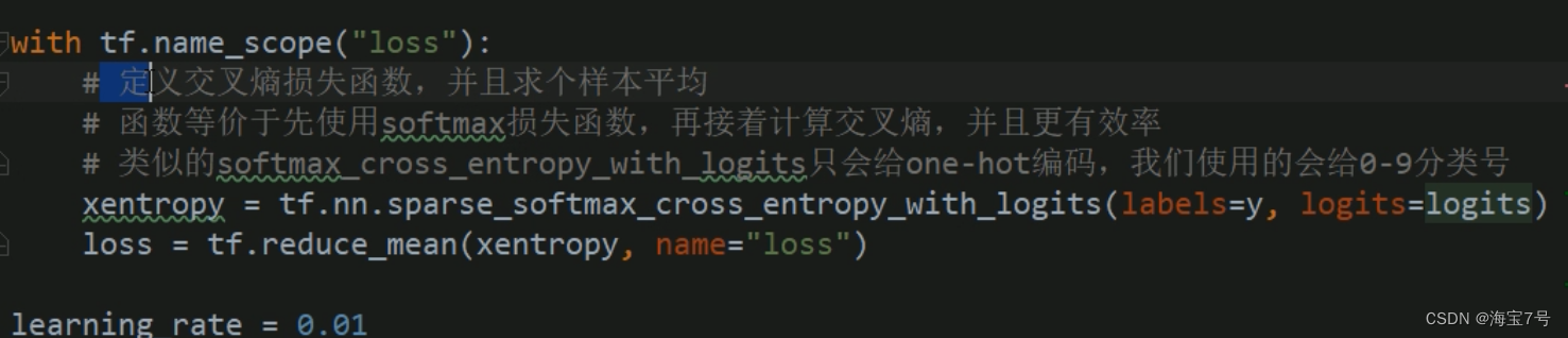
with tf.name_scope("loss"):
# Define the cross entropy loss function , And average a sample
# Function is equivalent to using first softmax Loss function , And then we calculate the cross entropy , And more efficient
# Allied softmax_cross_entropy_with_logits Only for one-hot code , What we use will give 0-9 Classification number
xentropy = tf.nn.sparse_softmax_cross_entropy_with_logits(labels=y, logits=logits)
loss = tf.reduce_mean(xentropy, name="loss")
learning_rate = 0.01
with tf.name_scope("train"):
optimizer = tf.train.GradientDescentOptimizer(learning_rate)
training_op = optimizer.minimize(loss)
with tf.name_scope("eval"):
# obtain logits The biggest one in it 1 Bit and y Compare whether the categories are the same , return True perhaps False A set of values
correct = tf.nn.in_top_k(logits, y, 1)
accuracy = tf.reduce_mean(tf.cast(correct, tf.float32))
init = tf.global_variables_initializer()
saver = tf.train.Saver()
# Calculation chart stage
mnist = input_data.read_data_sets("MNIST_data_bak/")
n_epochs = 400
batch_size = 50
with tf.Session() as sess:
init.run()
for epoch in range(n_epochs):
for iteration in range(mnist.train.num_examples // batch_size):
X_batch, y_batch = mnist.train.next_batch(batch_size)
sess.run(training_op, feed_dict={
X: X_batch, y: y_batch})
acc_train = accuracy.eval(feed_dict={
X: X_batch, y: y_batch})
acc_test = accuracy.eval(feed_dict={
X: mnist.test.images,
y: mnist.test.labels})
print(epoch, "Train accuracy:", acc_train, "Test accuracy:", acc_test)
save_path = saver.save(sess, "./my_dnn_model_final.ckpt")
'''
# Use model forecast
with tf.Session as sess:
saver.restore(sess, "./my_dnn_model_final.ckpt")
X_new_scaled = [...]
Z = logits.eval(feed_dict={
X: X_new_scaled})
y_pred = np.argmax(Z, axis=1) # See which category is the largest
'''
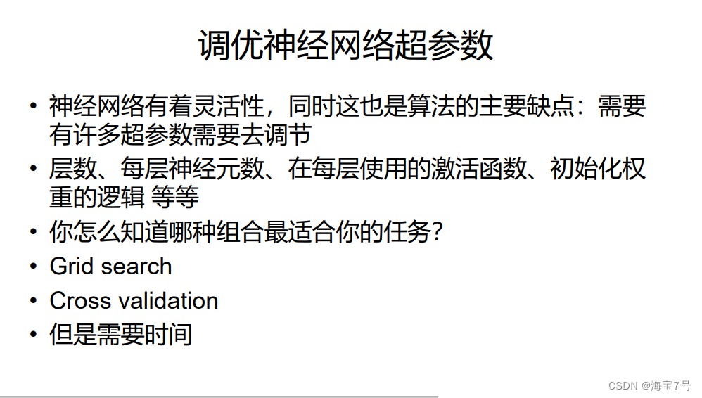
Tuning neural network superparameters
• Number of hidden layers
• For many questions , You can start with just one hidden layer , You can get good results , For example, for complex problems, we can
Just use enough neurons on the hidden layer , For a long time, people were satisfied and did not explore deep Neural Networks
• But the deep neural network has higher parameter efficiency , The number of neurons can be exponentially reduced , And train faster !
• It's like drawing a forest directly will be slow , But if you draw branches , Copy and paste branches into trees , Copying and pasting trees into forests is very
fast . The real world is usually this hierarchical structure ,DNN Is to use this advantage
• The previous hidden layer builds a low-level structure , Lines that form various shapes and directions , The middle hidden layer combines low-level structures , For example, Fang
block 、 circular , The later hidden layer and output layer form a more advanced structure , Like the face
• Not only does this hierarchical structure help DNN Convergence is faster , At the same time, it increases the reusability to new data sets , for example , If you have already trained
A neural network to recognize faces , Now you want to train a new network to recognize hairstyles , You can reuse the previous layers , Just don't go
Random initialization Weights and biases, You can assign the weight values of the previous layers in the first network to the new network as initialization , Then start training
• In this way, the network does not have to train the low-level network structure from the original , It only needs to train high-rise structures .
• For many questions , One or two hidden layers are enough ,MNIST You can achieve 97% When using a hidden layer of hundreds of neurons
, achieve 98% Use two hidden layers , For more complex problems , You can gradually increase the hidden layer , Until the training set is fitted .
• Very complex tasks such as image classification and speech recognition , It needs dozens or even hundreds of floors , But not all are connected , And they need to be big
The amount of data , however , You rarely need to train from scratch , It is very convenient to reuse some classic networks of similar services that have been trained in advance .
That way, the training will be much faster and will not require much data .
• The number of neurons in each hidden layer
• The number of neurons in the input layer and the output layer can be easily determined , According to the demand , such as MNIST Input layer 28*28=784, Output layer 10
• The usual practice is that there are fewer and fewer neurons in each hidden layer , For example, the first hidden layer 300 Neurons , The second hidden layer 100 Neurons , But , Now the number of neurons in each hidden layer is more the same , For example, all of them are 150 individual , In this way, there is less need to adjust the super parameters , Just like looking for the number of hidden layers before , You can gradually increase the number until it is over fitted , Finding the perfect number is more or black Technology
• The simple way is to choose more layers and neurons than you actually need , And then use early stopping To prevent over fitting , also L1、L2 Regularization techniques , also dropout
adopt Regularization Prevent over fitting
Typical deep learning has hundreds of parameters , Sometimes even millions , from
For so many super parameters , The network has unimaginable degrees of freedom to adapt to large
Measure all kinds of complex data sets . But this flexibility also means a tendency to train
Practice set fitting .
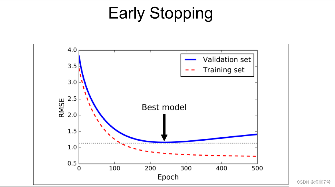
Early Stopping
Reference resources :https://www.jianshu.com/p/9ab695d91459
https://keras.io/callbacks/#earlystopping
https://zhuanlan.zhihu.com/p/186458993
https://tensorflow.google.cn/guide/migrate/early_stopping
To avoid overfitting , Often need to use early-stopping, That is in your loss When approaching convergence , You can stop training in advance
EarlyStopping yes Callbacks A kind of ,callbacks Used to specify in each epoch What is the specific operation to be performed at the beginning and the end .Callbacks There are some set interfaces in , You can use it directly , Such as ’acc’, 'val_acc’, ’loss’ and ’val_loss’ wait .
EarlyStopping It's used to stop training in advance callbacks. In particular , Can be achieved when training set loss It's not diminishing ( That is, the degree of reduction is less than a certain threshold ) Stop training when .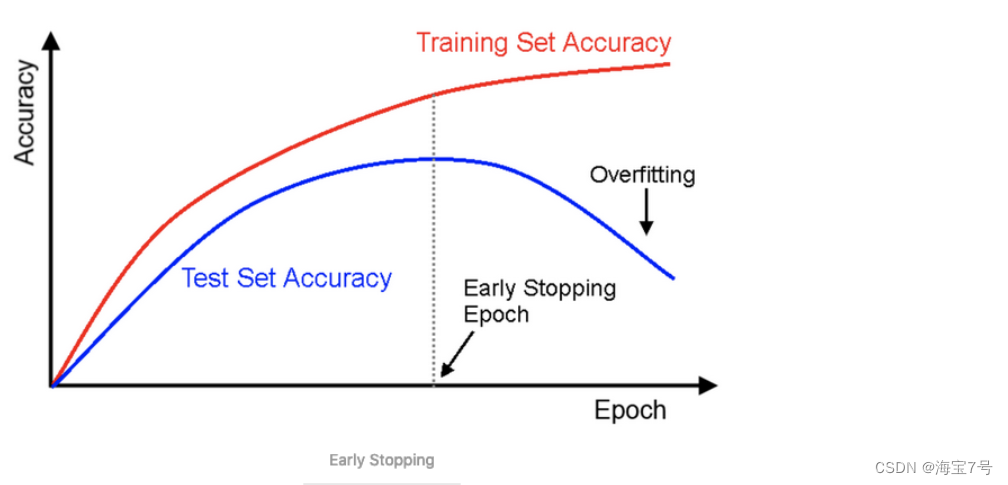
To prevent over fitting on the training set , A good method is early
stopping, Interrupt the training when the descent starts on the verification set
• One way to use TensorFlow To achieve , It's interval, such as every 50
steps, Evaluate the model on the validation set , Then save the snapshot if you lose
The output performance is better than the previous snapshot , Remember to iterate the last time you save a snapshot
Of steps The number of , When they arrive in step Of limit Times ,restore most
The last winning snapshot
• Even though early stopping The actual work is done well , You can still get better
When combined with other regularization techniques .
Relevant code parameters 
L1 L2 Regularization processing
• Use L1 and L2 Regularization to restrict neural network connections weights The weight
• A way to use TensorFlow To do regularization is to add the appropriate regularization term to the loss function .
But if there are many layers , The above method is not very convenient , Fortunately, ,
TensorFlow Provides a better choice , Many functions, such as get_variable() perhaps fully_connected() Accept one *_regularizer Parameters , Can pass anything with weights Is the parameter , Return the function corresponding to the regularization loss ,1_regularizer(),l2_regularizer() and l1_l2_regularizer() Function returns this function .
The above code neural network has two hidden layers , An output layer , At the same time
Create nodes in the graph to calculate the weight of each layer L1 We're losing ,
TensorFlow Automatically add these nodes to a special containing all regular
Set of chemical losses . You just need to add these regularization losses to the overall loss
Missing Center , Don't forget to add the regularization loss to the overall loss , otherwise
They will be ignored .
Dropout operation
• keep_prob Is the retained proportion ,1-keep_prob yes dropout rate
• When training , hold is_training Set to True, When it comes to testing , set up
Set as False.
Principle diagram 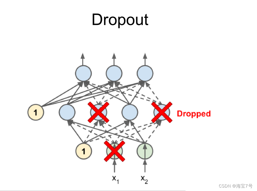
The code is as follows :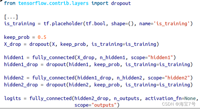
Tuning the activation function of neural network hyperparameters
• In most cases, the activation function uses ReLU Activation function , This activation function
Faster calculation , And the gradient descent will not get stuck plateaus, And for big
The input value of , It won't saturate , Opposite contrast logistic function and
hyperbolic tangent function, Will be saturated in 1
• For the output layer ,softmax Activation function is usually a good choice for fractional
Class task , Because categories are mutually exclusive , For the return
service , Do not use activation functions at all
• Activation function
• In most cases, the activation function uses ReLU Activation function , This activation function
Faster calculation , And the gradient descent will not get stuck plateaus, And for big
The input value of , It won't saturate , Opposite contrast logistic function and
hyperbolic tangent function, Will be saturated in 1
• For the output layer ,softmax Activation function is usually a good choice for fractional
Class task , Because categories are mutually exclusive , For the return
service , Do not use activation functions at all
• In most cases, the activation function uses ReLU Activation function , This activation function
Faster calculation , And the gradient descent will not get stuck plateaus, And for big
The input value of , It won't saturate , Opposite contrast logistic function and
hyperbolic tangent function, Will be saturated in 1
• For the output layer ,softmax Activation function is usually a good choice for fractional
Class task , Because categories are mutually exclusive , For the return
service , Do not use activation functions at all .
ReLU Activation function
Rectified Linear Units
• ReLU Calculate that the linear function is nonlinear , If it is greater than 0 It's the result , otherwise
Namely 0
• The response of biological neurons looks like Sigmoid Activation function , all
The experts are Sigmoid I got stuck for a long time , But it turns out ReLU Caigeng
Suitable for artificial neural network , This is a misunderstanding of simulated Biology .
Several activation functions and their derivatives :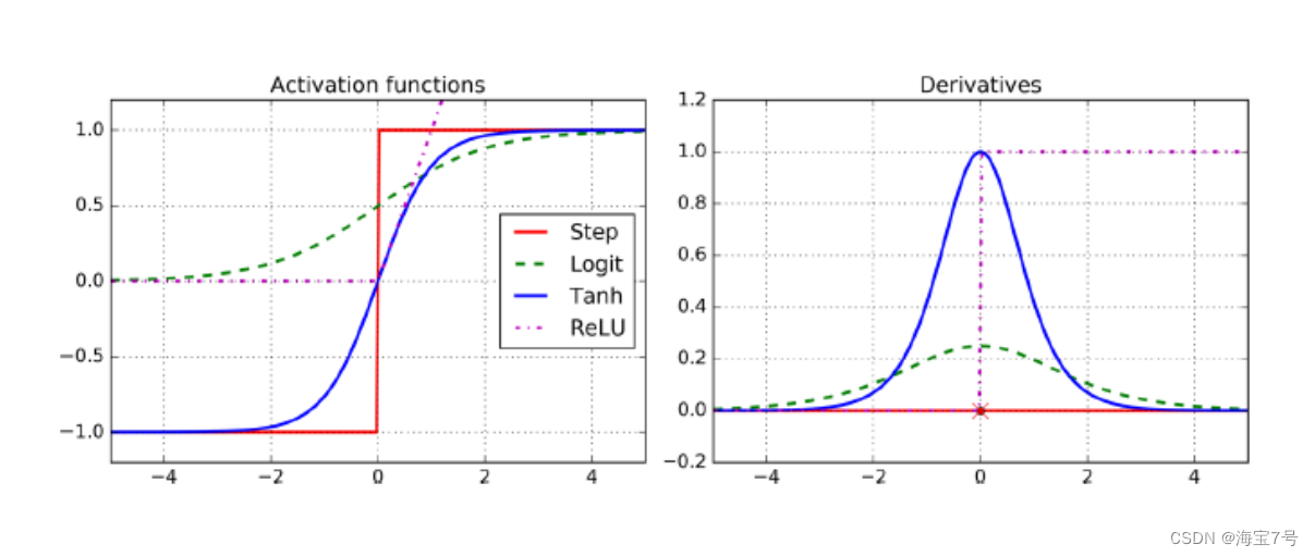
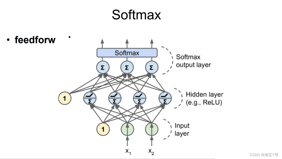
Softmax Handle .
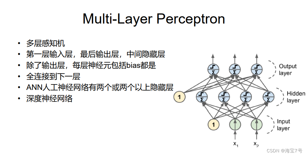
Multilayer perceptron is usually used for classification problems , Two classification
• There are also many times it will be used for multi classification , You need to change the activation function of the output layer
Become a shared softmax function
• The output becomes a probability value used to evaluate which category it belongs to
The data increases
• Generate some new training samples from the existing data , Manually increase the training set , This will reduce over fitting
• For example, if your model is a classified mushroom picture , You can translate slightly , rotate , Change size , Then add these changed pictures to the training set , This allows the model to withstand location , Direction , The impact of size , If you want to use the model, you can withstand the influence of light conditions , You can produce many pictures with different contrast , Suppose mushrooms are symmetrical , You can also flip the picture horizontally
As shown in the figure :
• TensorFlow Provide some image operators , for example transposing(shifting),> rotating,resizing,flipping,cropping,adjusting brightness,> contrast,saturation,hue
result :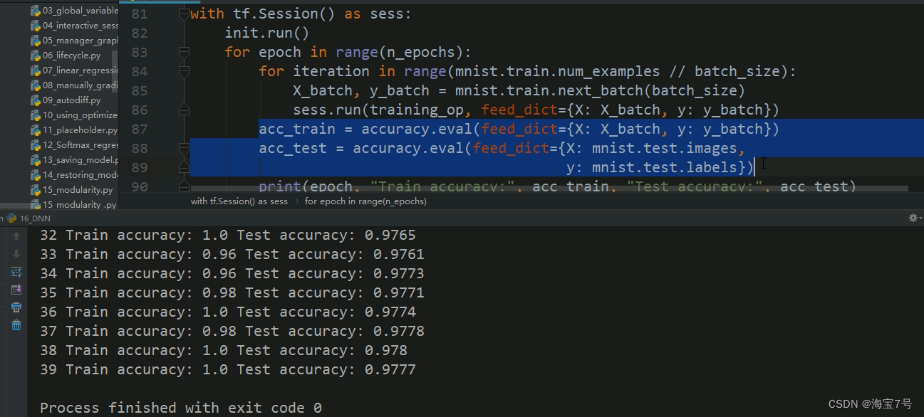
To be continued —>>>> Preface
边栏推荐
- Setting up Oracle datagurd environment
- 实现CNN图像的识别和训练通过tensorflow框架对cifar10数据集等方法的处理
- 编程内功之编程语言众多的原因
- Kivy教程之 盒子布局 BoxLayout将子项排列在垂直或水平框中(教程含源码)
- 8皇后问题
- Universal dividend source code, supports the dividend of any B on the BSC
- Internet of things completion -- (stm32f407 connects to cloud platform detection data)
- Kivy教程之 如何自动载入kv文件
- In the promotion season, how to reduce the preparation time of defense materials by 50% and adjust the mentality (personal experience summary)
- File uploading and email sending
猜你喜欢
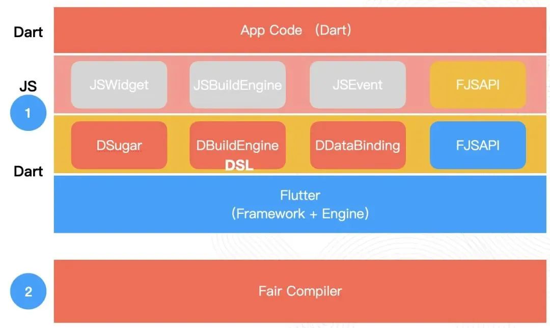
Flutter dynamic | fair 2.5.0 new version features
![[how to solve FAT32 when the computer is inserted into the U disk or the memory card display cannot be formatted]](/img/95/09552d33d2a834af4d304129714775.png)
[how to solve FAT32 when the computer is inserted into the U disk or the memory card display cannot be formatted]

The principle of human voice transformer

【历史上的今天】7 月 3 日:人体工程学标准法案;消费电子领域先驱诞生;育碧发布 Uplay
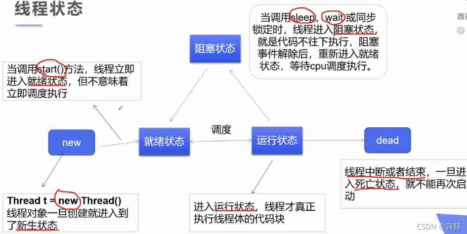
Detailed explanation of multithreading

PowerPoint tutorial, how to save a presentation as a video in PowerPoint?
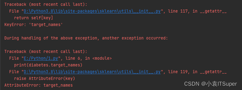
已解决(机器学习中查看数据信息报错)AttributeError: target_names

NFT新的契机,多媒体NFT聚合平台OKALEIDO即将上线
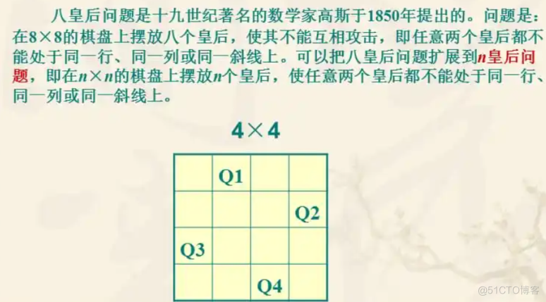
8皇后问题

MySQL installation, uninstallation, initial password setting and general commands of Linux
随机推荐
MySQL installation, uninstallation, initial password setting and general commands of Linux
已解决(机器学习中查看数据信息报错)AttributeError: target_names
Flink code is written like this. It's strange that the window can be triggered (bad programming habits)
SQL Injection (POST/Search)
Complete deep neural network CNN training with tensorflow to complete picture recognition case 2
刚毕业的欧洲大学生,就能拿到美国互联网大厂 Offer?
Flink SQL knows why (XV): changed the source code and realized a batch lookup join (with source code attached)
The R language GT package and gtextras package gracefully and beautifully display tabular data: nflreadr package and gt of gtextras package_ plt_ The winloss function visualizes the win / loss values
Logseq 评测:优点、缺点、评价、学习教程
R语言使用data函数获取当前R环境可用的示例数据集:获取datasets包中的所有示例数据集、获取所有包的数据集、获取特定包的数据集
Flink SQL knows why (16): dlink, a powerful tool for developing enterprises with Flink SQL
MapReduce实现矩阵乘法–实现代码
Task5: multi type emotion analysis
NFT新的契机,多媒体NFT聚合平台OKALEIDO即将上线
SwiftUI 开发经验之作为一名程序员需要掌握的五个最有力的原则
Father and basketball
JSON serialization case summary
Logseq evaluation: advantages, disadvantages, evaluation, learning tutorial
太阳底下无新事,元宇宙能否更上层楼?
服务器硬盘冷迁移后网卡无法启动问题