当前位置:网站首页>Linear programming of mathematical modeling (including Matlab code)
Linear programming of mathematical modeling (including Matlab code)
2022-07-03 01:00:00 【Yi EBA】
List of articles
Linear programming of mathematical modeling
1. Linear programming
1.1 matlab The standard form in

>> c = [-2;-3;5]; %  Equate to  c = [-2,-3,5]';  seek max Take the opposite
>> A = [-2,5,-1;1,3,1]; %  inequality
>> b = [-10;12]; %  inequality
>> Aeq = [1,1,1]; %  equation
>> beq = 7; %  equation
>> [x,fval] = linprog(c,A,b,Aeq,beq,zeros(3,1)); %  Get results


>> x

x =

    6.4286
    0.5714
         0

>> z = -fval

z =

   14.5714

%  explain : stay x1 x2 x3 = 6.4286 0.5714 0  Under the circumstances ,maxz = 14.5714
1.2 It can be transformed into a linear programming problem

Example :


Explain : Variable substitution , Turn it into a linear programming model :
c =

     1     2     3     4

>> c = [c,c]'

c =

     1
     2
     3
     4
     1
     2
     3
     4

>> Aeq = [1,-1,-1,1;1,-1,1,-3;1,-1,-2,3]

Aeq =

     1    -1    -1     1
     1    -1     1    -3
     1    -1    -2     3

>> Aeq = [Aeq,-Aeq]

Aeq =

     1    -1    -1     1    -1     1     1    -1
     1    -1     1    -3    -1     1    -1     3
     1    -1    -2     3    -1     1     2    -3

>> beq = [0;1;-1/2]

beq =

         0
    1.0000
   -0.5000

>> [uv,fval] = linprog(c,[],[],Aeq,beq,zeros(8,1));

Optimal solution found.

>> x = uv(1:4) - uv(5:end)

x =

    0.2500
         0
         0
   -0.2500

>> minz = fval

minz =

    1.2500

>>


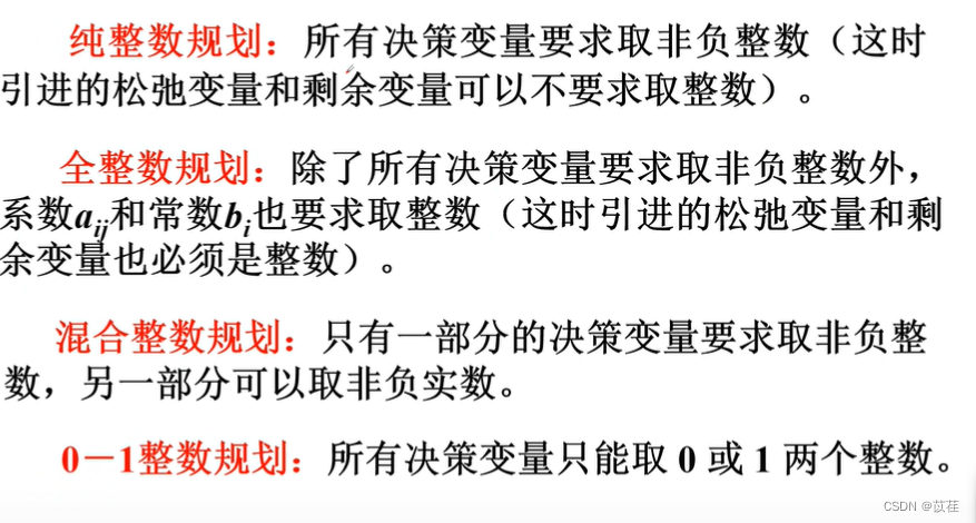
2. Integer programming
The integer of integer programming is only for decision variables , It has nothing to do with whether the optimal solution is an integer .


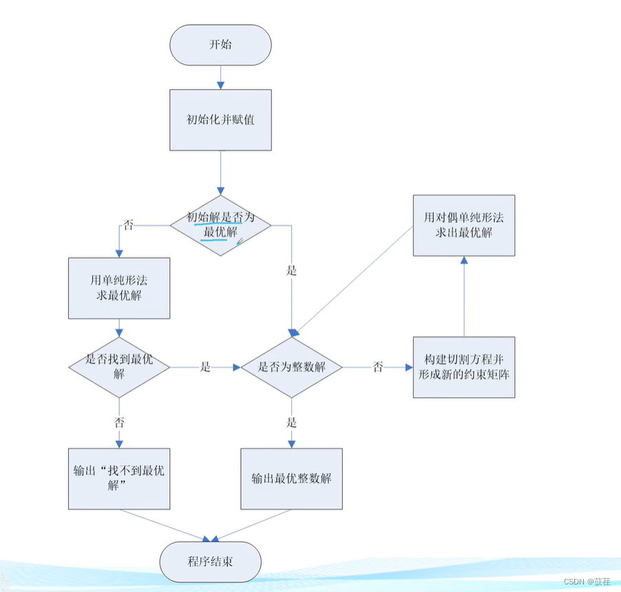
2.1 Branch and bound algorithm
Usually , Divide all feasible solution spaces into smaller and smaller subsets repeatedly
Set , It's called branching ; And calculate a target lower bound for the solution set in each subset ( For the minimum value problem ), This name
Delimit . After each branch , Those subsets whose bounds exceed the target value of the known feasible solution set will not be further branched , such , Many subsets may be disregarded , This is called pruning . This is the main idea of branch and bound method .
The branch and bound method can be used to solve pure integer or mixed integer programming problems .
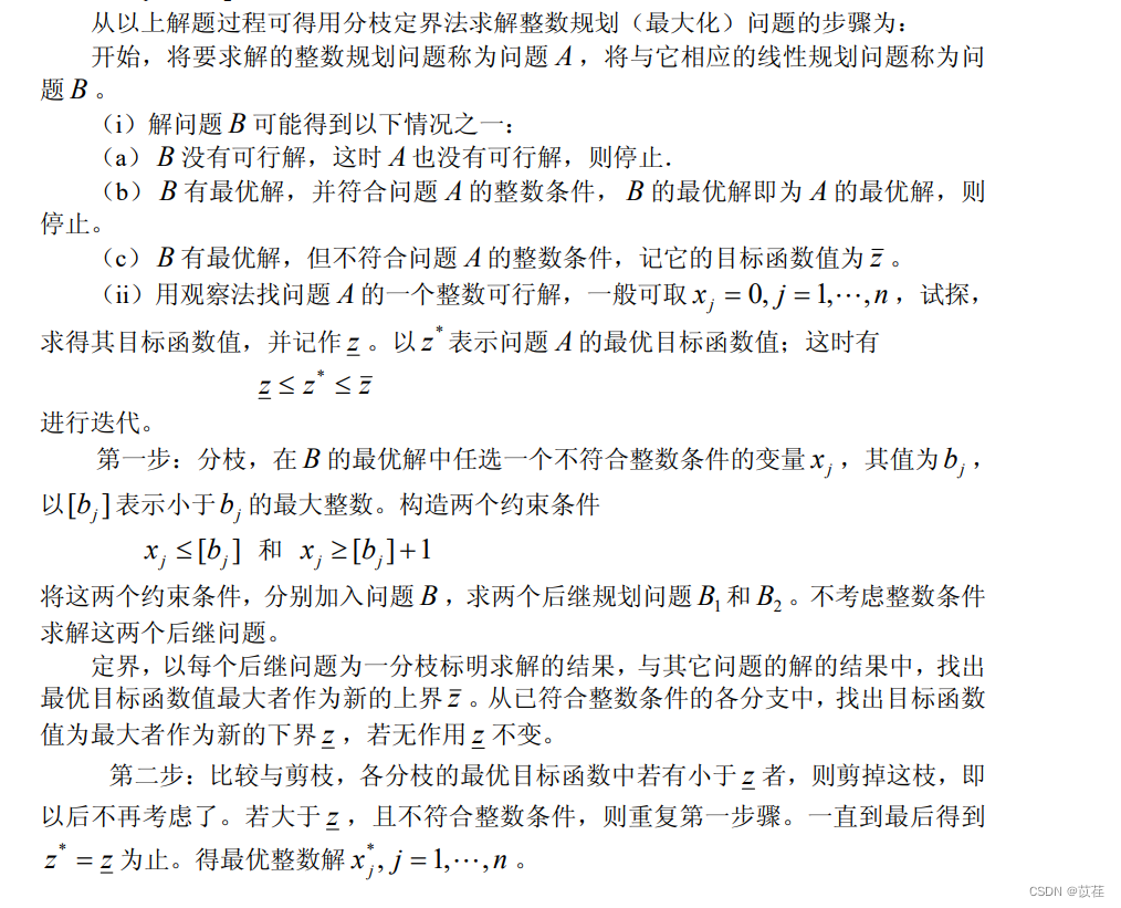
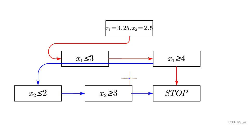
2.1.1 Example of branch and bound

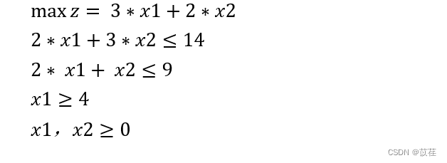
>> c = [-3;-2];
>> A = [2,3;2,1];
>> b = [14;9];
>> [x,fval] = linprog(c,A,b,[],[],zeros(2,1));

Optimal solution found.

>> x

x =

    3.2500
    2.5000

>> z = - fval

z =

   14.7500

>>
You can see ,x It's not an integer , Next, branch and bound :

>> [x,fval] = linprog(c,A,b,[],[],zeros(2,1),[3,inf]);

Optimal solution found.

>> x

x =

    3.0000
    2.6667

>> z = -fval

z =

   14.3333

>>
Continue to branch and bound :
>> [x,fval] = linprog(c,A,b,[],[],[4,0]);

Optimal solution found.

>> x

x =

    4.0000
    1.0000

>> z = -fval

z =

   14.0000
14.3333 Than 14.0000 Big , So in x1≤3 Next, branch and bound :
>> [x,fval] = linprog(c,A,b,[],[],zeros(2,1),[3,2]);

Optimal solution found.

>> x

x =

     3
     2

>> z = -fval

z =

    13

>>
Continue to branch and bound :
>> [x,fval] = linprog(c,A,b,[],[],[0,3],[3,inf]);

Optimal solution found.

>> x

x =

    2.5000
    3.0000

>> z = -fval

z =

   13.5000

>>
So the optimal solution of integer programming is 14.
2.1.2 matlab Code implementation
branchbound.m
function [newx,newfval,status,newbound] = branchbound(f,A,B,I,x,fval,bound,Aeq,Beq,lb,ub,e)

%  Branch and bound method to solve integer programming
% f,A,B,Aeq,Beq,lb,ub Same as linear programming
% I A vector that limits variables to integers
% x Is the initial solution ,fval For the initial value

options = optimset('display','off');
[x0,fval0,status0]=linprog(f,A,B,Aeq,Beq,lb,ub,[],options);

% Final exit condition in recursion
% If there is no solution or the solution is larger than the existing upper bound, the original solution is returned
if status0 <= 0 || fval0 >= bound
    newx = x;
    newfval = fval;
    newbound = bound;
    status = status0;
    return;
end

% Whether it is an integer solution , If it is an integer solution, it returns
intindex = find(abs(x0(I) - round(x0(I))) > e);
if isempty(intindex) % Judge whether it is a null value
    newx(I) = round(x0(I));
    newfval = fval0;
    newbound = fval0;
    status = 1;
    return;
end

% When there is a non integral feasible solution , Then branch solution
% At this point, there must be an integer solution or an empty solution
% Find the first variable that does not meet the integer requirements
n = I(intindex(1));
addA = zeros(1,length(f));
addA(n) = 1;
% Construct the first branch  x<=floor(x(n))
A = [A;addA];
B = [B,floor(x(n))];% Rounding down
[x1,fval1,status1,bound1] = branchbound(f,A,B,I,x0,fval0,bound,Aeq,Beq,lb,ub,e);
A(end,:) = [];
B(:,end) = [];
% The first branch of the solution , If it is a better solution, replace , If not, leave it as it is

status = status1;
if status1 > 0 && bound1 < bound
    newx = x1;
    newfval = fval1;
    bound = fval1;
    newbound = bound1;
else
    newx = x0;
    newfval = fval0;
    newbound = bound;
end

% Construct the second branch
A = [A;-addA];
B = [B,-ceil(x(n))];% Rounding up
[x2,fval2,status2,bound2] = branchbound(f,A,B,I,x0,fval0,bound,Aeq,Beq,lb,ub,e);
A(end,:) = [];
B(:,end) = [];

% The second branch of the solution , And compare it with the first branch , If better, replace
if status2 > 0 && bound2 < bound
    status = status2;
    newx = x2;
    newfval = fval2;
    newbound = bound2;
end
intprog.m
function [x,fval,status] = intprog(f,A,B,I,Aeq,Beq,lb,ub,e)
% Integer programming solving function  intprog()
%      among  f Is the objective function vector
%     A and B For inequality constraints  Aeq And Beq For equality constraints
%     I Is an integer constraint
%     lb And ub They are the lower bound and upper bound of variables
%     x For the best solution ,fval Is the optimal value
% Example :
%        maximize 20 x1 + 10 x2
%        S.T.
% 	             5 x1 + 4 x2 <=24
%                2 x1 + 5 x2 <=13
%                   x1, x2 >=0
%                   x1, x2 Is an integer
% f=[-20, -10];
% A=[ 5  4; 2 5];
% B=[24; 13];
% lb=[0 0];
% ub=[inf inf];
% I=[1,2];
% e=0.000001;
% [x v s]= IP(f,A,B,I,[],[],lb,ub,,e)
% x = 4     1  v = -90.0000   s = 1

%  Control input parameters
if nargin < 9, e = 0.00001;
   if nargin < 8, ub = [];
      if nargin < 7, lb = [];
         if nargin < 6, Beq = [];
            if nargin < 5, Aeq = [];
               if nargin < 4, I = [1:length(f)];
               end, end, end, end, end, end

% Solve the linear programming corresponding to integer programming , Judge whether there is a solution
options = optimset('display','off');
[x0,fval0,exitflag] = linprog(f,A,B,Aeq,Beq,lb,ub,[],options);
if exitflag < 0
    disp(' There is no suitable integer solution ');
    x = x0;
    fval = fval0;
    status = exitflag;
    return;
else
    % The branch and bound method is used to solve
    bound = inf;
    [x,fval,status] = branchbound(f,A,B,I,x0,fval0,bound,Aeq,Beq,lb,ub,e);
end
Branch and bound process :
2.1.3 intlinprog Function to solve integer programming

>> c = [-40;-90];
>> A = [9,7;7,20];
>> b = [56;70];
>> [x,fval] = intlinprog(c,[1 2],A,b,[],[],zeros(2,1));
>> x

x =

    4.0000
    2.0000

>> -fval

ans =

   340

x = intlinprog(f,intcon,A,b,Aeq,beq,lb,ub): Compared to the function linprog One more parameter intcon, Used to calibrate the position of integer variables :x1、x2 Integers , namely intcon = [1 2].
2.2 Cut plane algorithm
Explain : Two inequalities , Here we introduce two relaxation variables x3 and x4;

2.2.1 matlab Implementation code
function  [intx,intf] = DividePlane(A,c,b,baseVector)
% function : Solve integer programming by cutting plane method
% Invocation format :[intx,intf]=DividePlane(A,c,b,baseVector)
% among , A: Constraint matrix ;
%      c: Objective function coefficient vector ;
%      b: Constrain the right vector ;
%      baseVector: Initial basis vector ;
%      intx: The independent variable value when the objective function takes the maximum value ;
%      intf: The maximum value of the objective function ;
sz = size(A);
nVia = sz(2);% Get how many decision variables
n = sz(1);% Get how many constraints
xx = 1:nVia;

if length(baseVector) ~= n
    disp(' The number of base variables should be equal to the number of rows of the constraint matrix !');
    mx = NaN;
    mf = NaN;
    return;
end

M = 0;
sigma = -[transpose(c) zeros(1,(nVia-length(c)))];
xb = b;

% First, use the simplex method to find the optimal solution
while 1
    [maxs,ind] = max(sigma);
%-------------------- Use the simplex method to find the optimal solution --------------------------------------
    if maxs <= 0   % When the inspection numbers are less than 0 when , Find the optimal solution .
        vr = find(c~=0 ,1,'last');
        for l=1:vr
            ele = find(baseVector == l,1);
            if(isempty(ele))
                mx(l) = 0;
            else
                mx(l)=xb(ele);
            end
        end
        if max(abs(round(mx) - mx))<1.0e-7  % Determine whether the optimal solution is an integer solution , If it's an integer solution .
            intx = mx;
            intf = mx*c;
            return;
        else  % If the optimal solution is not an integer solution , Construction of cutting equation
            sz = size(A);
            sr = sz(1);
            sc = sz(2);
            [max_x, index_x] = max(abs(round(mx) - mx));
            [isB, num] = find(index_x == baseVector);
            fi = xb(num) - floor(xb(num));
            for i=1:(index_x-1)
                Atmp(1,i) = A(num,i) - floor(A(num,i));
            end
            for i=(index_x+1):sc
                Atmp(1,i) = A(num,i) - floor(A(num,i));
            end

            Atmp(1,index_x) = 0; % Construct the initial table of dual simplex method
            A = [A zeros(sr,1);-Atmp(1,:) 1];
            xb = [xb;-fi];
            baseVector = [baseVector sc+1];
            sigma = [sigma 0];

            %------------------- Iterative process of dual simplex method ----------------------
            while 1
                %----------------------------------------------------------
                if xb >= 0    % Judge if the right end vectors are greater than 0, Find the optimal solution
                    if max(abs(round(xb) - xb))<1.0e-7   % If the integer solution is obtained by the dual simplex method , Then the optimal integer solution is returned
                        vr = find(c~=0 ,1,'last');
                        for l=1:vr
                            ele = find(baseVector == l,1);
                            if(isempty(ele))
                                mx_1(l) = 0;
                            else
                                mx_1(l)=xb(ele);
                            end
                        end
                        intx = mx_1;
                        intf = mx_1*c;
                        return;
                    else   % If the optimal solution obtained by the dual simplex method is not an integer solution , Continue to add cutting equations
                        sz = size(A);
                        sr = sz(1);
                        sc = sz(2);
                        [max_x, index_x] = max(abs(round(mx_1) - mx_1));
                        [isB, num] = find(index_x == baseVector);
                        fi = xb(num) - floor(xb(num));
                        for i=1:(index_x-1)
                            Atmp(1,i) = A(num,i) - floor(A(num,i));
                        end
                        for i=(index_x+1):sc
                            Atmp(1,i) = A(num,i) - floor(A(num,i));
                        end
                        Atmp(1,index_x) = 0;  % The initial table of the next dual simplex iteration
                        A = [A zeros(sr,1);-Atmp(1,:) 1];
                        xb = [xb;-fi];
                        baseVector = [baseVector sc+1];
                        sigma = [sigma 0];
                        continue;
                    end
                else   % If the right vector is not all greater than 0, Then carry out the process of changing base variables of dual simplex method
                    minb_1 = inf;
                    chagB_1 = inf;
                    sA = size(A);
                    [br,idb] = min(xb);
                    for j=1:sA(2)
                        if A(idb,j)<0
                            bm = sigma(j)/A(idb,j);
                            if bm<minb_1
                                minb_1 = bm;
                                chagB_1 = j;
                            end
                        end
                    end
                    sigma = sigma -A(idb,:)*minb_1;
                    xb(idb) = xb(idb)/A(idb,chagB_1);
                    A(idb,:) = A(idb,:)/A(idb,chagB_1);
                    for i =1:sA(1)
                        if i ~= idb
                            xb(i) = xb(i)-A(i,chagB_1)*xb(idb);
                            A(i,:) = A(i,:) - A(i,chagB_1)*A(idb,:);
                        end
                    end
                    baseVector(idb) = chagB_1;
                end
              %------------------------------------------------------------
            end
            %-------------------- Iterative process of dual simplex method ---------------------
        end
    else     % If the inspection number is not less than 0 Of , Then carry out the iteration process of simplex algorithm
        minb = inf;
        chagB = inf;
        for j=1:n
            if A(j,ind)>0
                bz = xb(j)/A(j,ind);
                if bz<minb
                    minb = bz;
                    chagB = j;
                end
            end
        end
        sigma = sigma -A(chagB,:)*maxs/A(chagB,ind);
        xb(chagB) = xb(chagB)/A(chagB,ind);
        A(chagB,:) = A(chagB,:)/A(chagB,ind);
        for i =1:n
            if i ~= chagB
                xb(i) = xb(i)-A(i,ind)*xb(chagB);
                A(i,:) = A(i,:) - A(i,ind)*A(chagB,:);
            end
        end
        baseVector(chagB) = ind;
    end
    M = M + 1;
    if (M == 1000000)
        disp(' No optimal solution found !');
        mx = NaN;
        minf = NaN;
        return;
    end
end
2.2.2 Application of cutting plane algorithm
>> c = [-1;-1]; %  Do not add slack variables
>> A = [-1 1 1 0;3 1 0 1]; %  Add the relaxation variable
>> b = [1;4];
>> [x fval] = DividePlane(A,c,b,[3 4]); %  Relax variables  3 4
>> x

x =

    1.0000    1.0000

>> maxz = -fval

maxz =

     2

>>
2.3 hungarian algorithm (0-1 planning )
0-1 The planning problem can also be seen as an interval [0,1] Integer programming of , The following use intlinprog Function to calculate :

>> c = [-3 2 -5]';
>> A = [1 2 -1;1 4 1];
>> b = [2;4];
>> c = [-3 2 -5]';
>> A = [1 2 -1;1 4 1;1 1 0;0 4 1];
>> b = [2;4;3;6];
>> [x fval] = intlinprog(c,[1 2 3],A,b,[],[],zeros(3,1),ones(3,1));
>> x

x =

     1
     0
     1

>> maxz = -fval

maxz =

     8

>>
Hungarian algorithm solves 0-1 Programming problem :
2.3.1 Investment issues

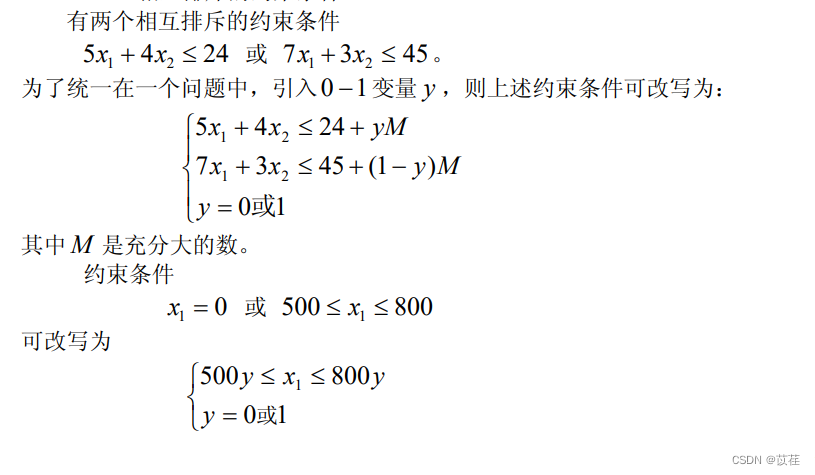
2.3.2 Mutually exclusive constraint problem

2.3.3 Fixed cost problem

2.3.4 Assignment problem

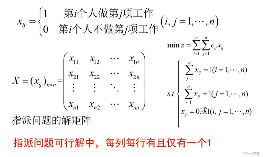
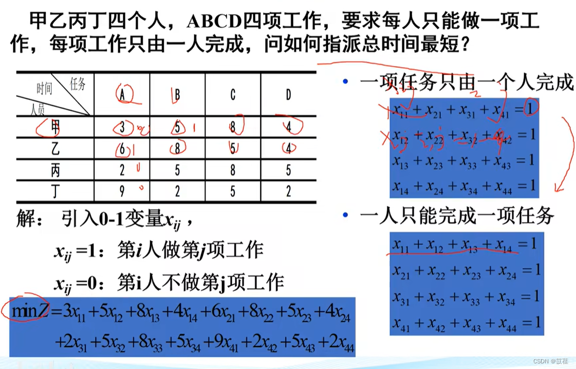
give an example
2.3.5 Nonstandard assignment problem

2.3.6 Hungarian algorithm description

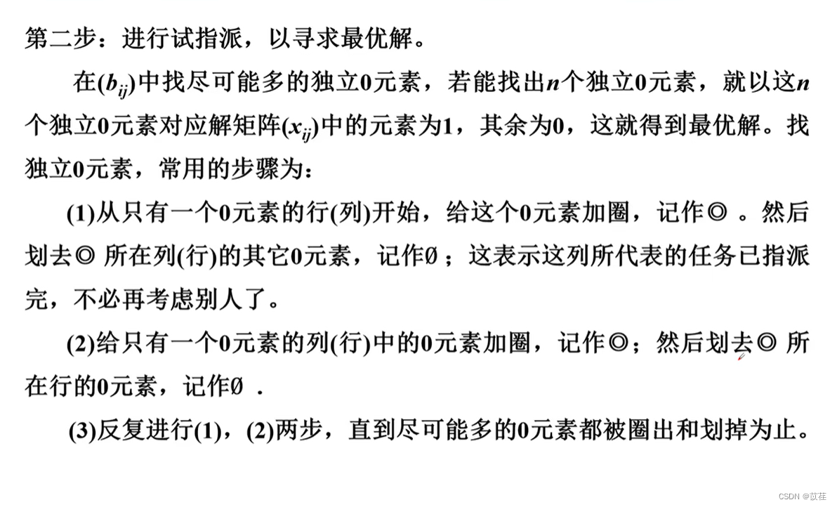
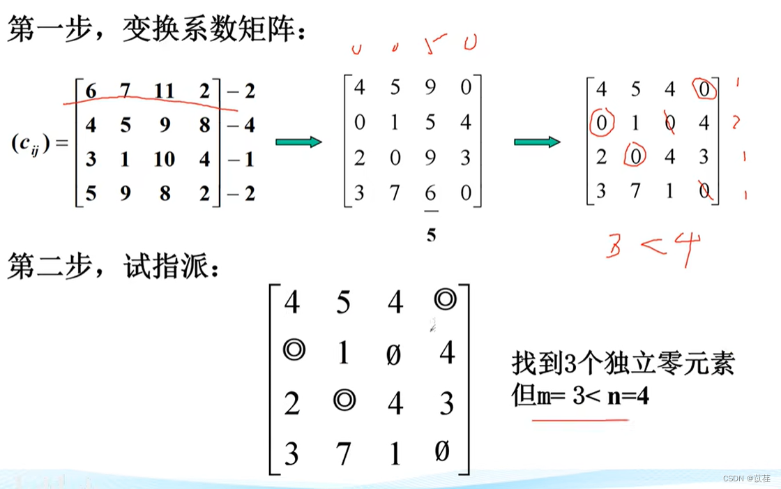
Find the minimum value in each line and subtract the minimum value from each element of the line , Find the minimum value in each column and subtract the minimum value from each element of the column , From only one 0 The line of the element begins , take 0 Element circle , Cross out this 0 Other elements in the column 0 Elements , Then look for only one 0 The row of the element , Repeat , In the business 0 When there is no element , There is only one 0 Columns of elements , loops , Cross out this 0 Other elements on the line 0 Elements .
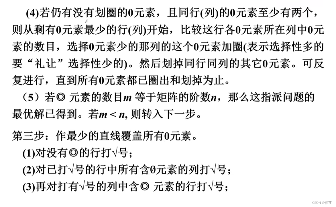
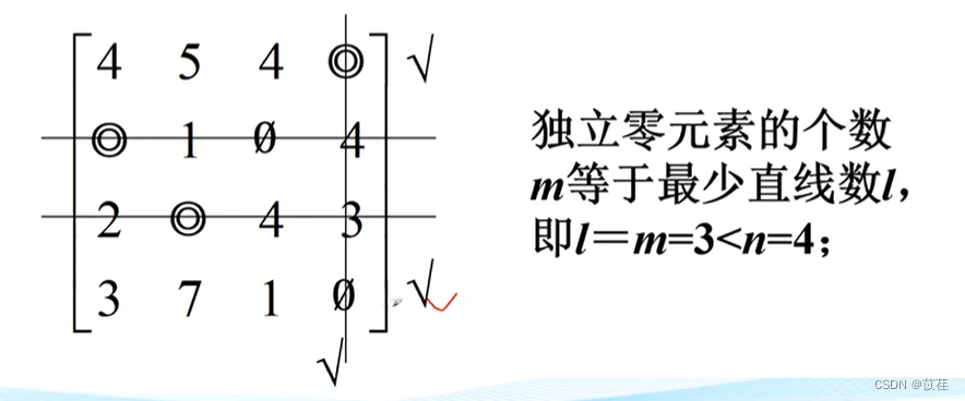
Last , If circled 0 The number of elements is less than the order n, Do the following :( Otherwise, find the solution )
Yes, there is no circle 0 The line type of elements √, Duel √ Cross out all in the line of 0 The column of the element is marked with √, Duel √ Columns of contain circles 0 The line of the element is marked √, Repeat the above 3 Step , Until we don't get a new hit √ The line of No .
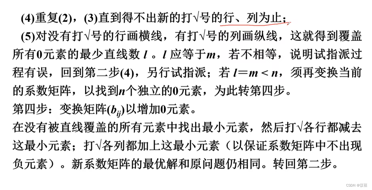
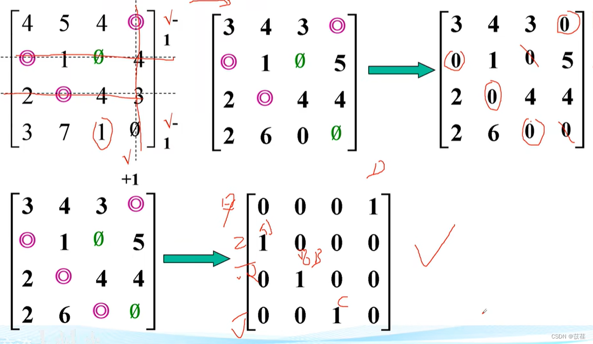
below , Yes, No √ Draw a horizontal line on the line , Duel √ Draw a vertical line on the column , So as to cover all 0 The minimum number of horizontal lines of an element , It should be equal to circle 0 Number of elements , Then proceed as follows , Transform the current matrix to increase 0 Elements , In order to find n Independent 0 Elements :
Find the minimum element value of all elements not covered by the line , Will hit √ Subtract the minimum element value from each line of , hit √ Add the minimum element value to each column of , Thus a new assignment matrix is obtained , Repeat the above with this new assignment matrix All steps , Until we find out n Independent 0 Element results .
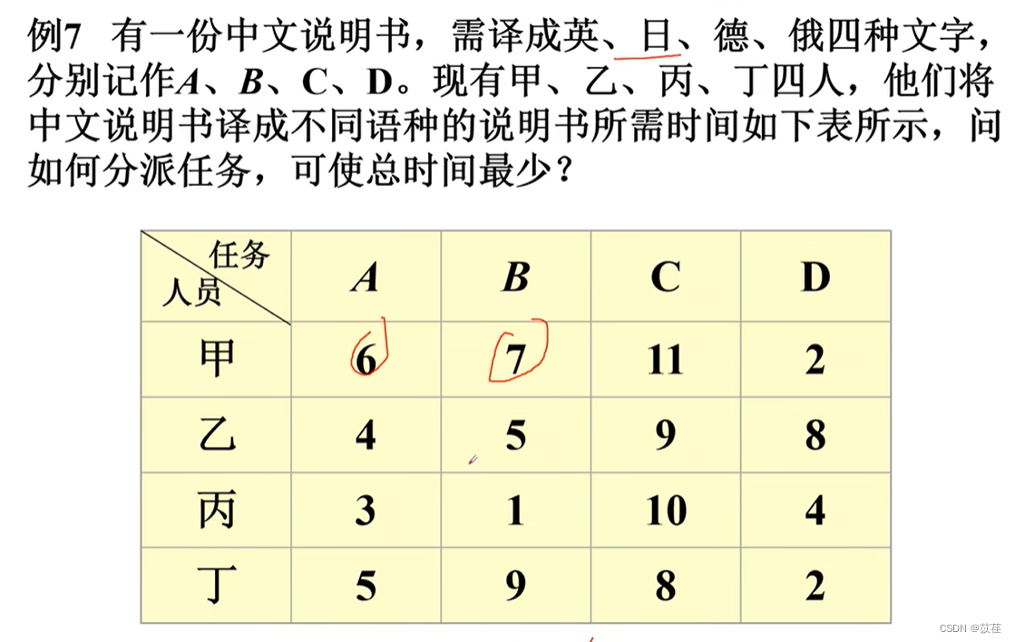
Example
Implementation steps
2.3.7 Hungarian algorithm code implementation
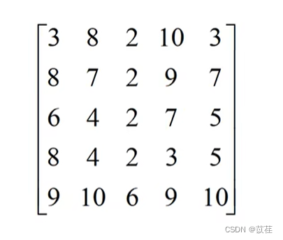
>> c = [3 8 2 10 3;8 7 2 9 7;6 4 2 7 5;8 4 2 3 5;9 10 6 9 10]

c =

     3     8     2    10     3
     8     7     2     9     7
     6     4     2     7     5
     8     4     2     3     5
     9    10     6     9    10

>> c = c(:); %  A matrix is converted into a vector
>> a = zeros(10,25);
>> for i = 1:5
a(i,(i-1)*5+1:5*i) = 1;
a(5+i,i:5:25) = 1;
end %  Loop transforms assignment problem into linear programming problem
>> b = ones(10,1); % 10 A constraint (5*2)
>> [x y] = linprog(c,[],[],a,b,zeros(25,1),ones(25,1));

Optimal solution found.

>> X = reshape(x,5,5)

X =

     0     0     0     0     1
     0     0     1     0     0
     0     1     0     0     0
     0     0     0     1     0
     1     0     0     0     0

>> opt = y

opt =

    21

>>
>> [x y] = linprog(-c,[],[],a,b,zeros(25,1),ones(25,1));

Optimal solution found.

>> X = reshape(x,5,5)

X =

     0     1     0     0     0
     0     0     0     1     0
     0     0     1     0     0
     1     0     0     0     0
     0     0     0     0     1

>> opt = -y

opt =

    37

>>

>> c = [6 7 11 2;4 5 9 8;3 1 10 4;5 9 8 2];
>> a = zeros(8,16);
>>  for i = 1:4
a(i,(i-1)*4+1:4*i) = 1;
a(4+i,i:4:16) = 1;
end
>> b = ones(8,1);
>>  [x y] = linprog(c,[],[],a,b,zeros(16,1),ones(16,1));

Optimal solution found.

>> X = reshape(x,4,4)

X =

     0     0     0     1
     1     0     0     0
     0     1     0     0
     0     0     1     0

>> opt = y

opt =

    15

>>
>> [x y]= linprog(-c,[],[],a,b,zeros(25,1),ones(25,1));

Optimal solution found.

>> X = reshape(x,5,5)

X =

     0     1     0     0     0
     0     0     0     1     0
     0     0     1     0     0
     1     0     0     0     0
     0     0     0     0     1

>> opt = -y

opt =

    37

>>
>> c = [6 7 11 2;4 5 9 8;3 1 10 4;5 9 8 2];
>> a = zeros(8,16);
>>  for i = 1:4
a(i,(i-1)*4+1:4*i) = 1;
a(4+i,i:4:16) = 1;
end
>> b = ones(8,1);
>>  [x y] = linprog(c,[],[],a,b,zeros(16,1),ones(16,1));

Optimal solution found.

>> X = reshape(x,4,4)

X =

     0     0     0     1
     1     0     0     0
     0     1     0     0
     0     0     1     0

>> opt = y

opt =

    15

>>
3. Reference material
《 Mathematical modeling algorithm and Application 》( Si keeping )《 Mathematical modeling algorithm and application problem solving 》( Si keeping )- >> bilibili Mathematical modeling learning tutorial
边栏推荐
- RK3568开发板评测篇(二):开发环境搭建
- Attributeerror: 'tuple' object has no attribute 'layer' problem solving
- [AUTOSAR II appl overview]
- Leetcode-1964: find the longest effective obstacle race route to each position
- 12_微信小程序之微信视频号滚动自动播放视频效果实现
- [AUTOSAR eight OS]
- 1.11 - 总线
- leetcode-849:到最近的人的最大距离
- 数学建模之线性规划(含MATLAB代码)
- 1.12 - Instructions
猜你喜欢

Vulkan performance and refinement
1.11 - 总线
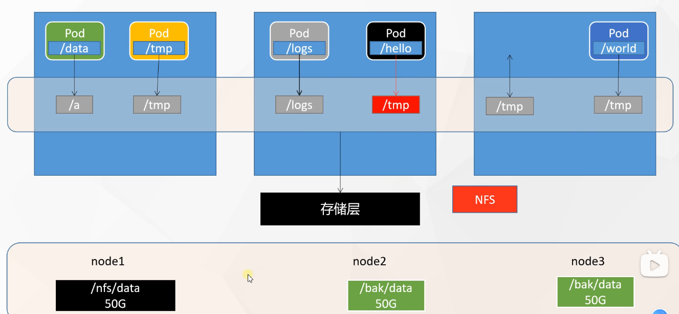
Kubernetes resource object introduction and common commands (V) - (NFS & PV & PVC)

【爱死机】《吉巴罗》被忽略的细节
kubernetes资源对象介绍及常用命令(五)-(NFS&PV&PVC)

Shell implements basic file operations (SED edit, awk match)
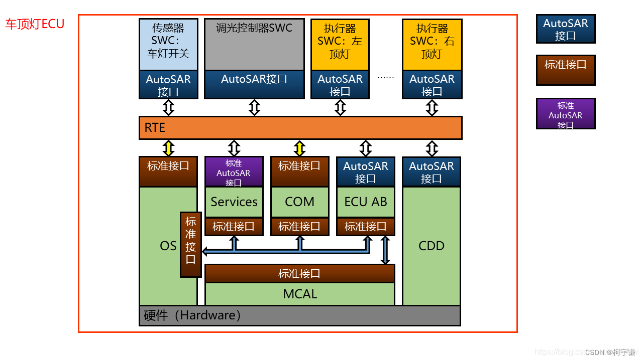
【AutoSAR 三 RTE概述】

Lu Zhe, chief scientist of Shiping information: building data and personnel centered security capabilities

Vulkan-实践第一弹

Web2.0的巨头纷纷布局VC,Tiger DAO VC或成抵达Web3捷径
随机推荐
拥抱平台化交付的安全理念
1038 Recover the Smallest Number
基于ARM RK3568的红外热成像体温检测系统
【AutoSAR 十三 NVM】
University of Toronto: Anthony coach | the conditions of deep reinforcement learning can induce dynamic risk measurement
世平信息首席科学家吕喆:构建以数据和人员为中心的安全能力
RISA rz/g2l processor introduction | frame diagram | power consumption | schematic diagram and hardware design guide
[overview of AUTOSAR three RTE]
How to find out the currently running version of Solr- How do I find out version of currently running Solr?
Is there a free text to speech tool to help recommend?
First hand evaluation of Reza electronics rz/g2l development board
465. 最优账单平衡 DFS 回溯
Key detection and sinusoidal signal output developed by Arduino
Initial order of pointer (basic)
Overlay of shutter (Pop-Up)
How to systematically learn machine learning
测试右移:线上质量监控 ELK 实战
线程的启动与优先级
[AUTOSAR twelve mode management]
Solve the cache problem of reactnative using WebView