当前位置:网站首页>[matlab] summary of conv, filter, conv2, Filter2 and imfilter convolution functions
[matlab] summary of conv, filter, conv2, Filter2 and imfilter convolution functions
2022-07-04 14:10:00 【Nirvana;】
【Matlab】conv、filter、conv2、filter2 and imfilter Function summary
1. conv function
effect :
1. Calculate one-dimensional vector convolution
u = [1 1 1];
v = [1 1 0 0 0 1 1];
w = conv(u,v)
2. Calculate polynomial multiplication through convolution
u = [1 0 1];
v = [2 7];
w = conv(u,v)
2. filter function
effect : One dimensional digital filter
y = filter(b,a,x) Use the numerator and denominator coefficients b and a Defined rational transfer function For input data x Filtering .
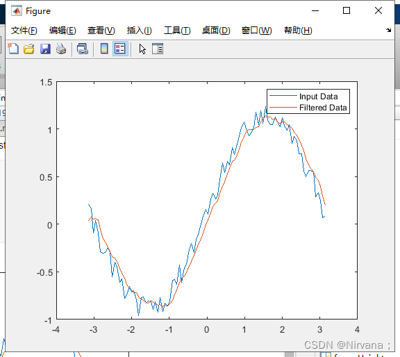
//  Moving average filter is a common method for smoothing noisy data .
t = linspace(-pi,pi,100);
rng default  %initialize random number generator
x = sin(t) + 0.25*rand(size(t));
windowSize = 5;
b = (1/windowSize)*ones(1,windowSize);
a = 1;
y = filter(b,a,x);
plot(t,x)
hold on
plot(t,y)
legend('Input Data','Filtered Data')
3. conv2 function
effect : Two dimensional convolution
A = rand(3);
B = rand(4);
C = conv2(A,B)
conv2 function
1、 usage
C=conv2(A,B,shape); % Convolution filtering
A: The input image ,B: Convolution kernel
Assumed input image A The size is ma x na, Convolution kernel B The size is mb x nb, be
When shape=full when , Return all two-dimensional convolution results , Return C The size is (ma+mb-1)x(na+nb-1)
shape=same when , Return and A The central part of the convolution of the same size
shape=valid when , Do not consider boundary zero filling , That is, as long as there is a boundary complement of zero, those involved in the operation are rounded off , return C The size is (ma-mb+1)x(na-nb+1)
2、 Implementation steps
Assumed input image A The size is ma x na, The convolution kernel size is mb x nb, be MATLAB Of conv2 The function implementation process is as follows :
a、 Zero the input image , Before the first line and after the last line mb-1 That's ok , Before the first column and after the last column nb-1 Column ( Be careful conv2 Other boundary supplement options are not supported , The function always fills the input with zero ).
b、 About the center of convolution kernel , Rotating convolution kernel 180 degree .
c、 Sliding convolution kernel , The center of the convolution kernel is located in each element of the image matrix .
d、 Multiply the rotated convolution kernel by the corresponding matrix elements and then sum .
4. filter2 function
1、 usage
B = filter2(h,A,shape) ; % relevant (correlation) wave filtering
- A: The input image ,h: Related nuclear
- Assumed input image A The size is ma x na, Related nuclear h The size is mb x nb, be
When shape=full when , Return all two-dimensional convolution results , Return B The size is (ma+mb-1)x(na+nb-1) - shape=same when , Return and A The central part of the convolution of the same size
- shape=valid when , Do not consider boundary zero filling , That is, as long as there is a boundary complement of zero, those involved in the operation are rounded off , return B The size is (ma-mb+1)x(na-nb+1)
2、 Implementation steps
Assumed input image A The size is ma x na, Related nuclear h The size is mb x nb,MATLAB Of filter2 The implementation process of is as follows :
- a、 Zero the input image , Before the first line and after the last line mb-1 That's ok , Before the first column and after the last column nb-1 Column ( Be careful filter2 Other boundary supplement options are not supported , The function always fills the input with zero ).
- b、 Sliding correlation core , The center of the correlation kernel is located in each element of the image matrix .
- c、 Multiply the correlation kernel by the corresponding matrix elements and then sum
Be careful filter2 No nuclear 180° rotate , Directly correspond to multiply and add , This is related to filter2 Different .
5. imfilter function
1、 usage
B=imfilter(A,H,option1,option2,option3);
A: The input image ,H: Filter core
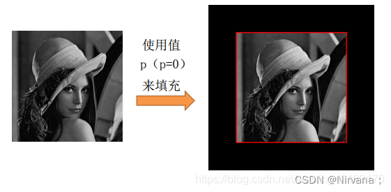
- option1: Boundary options , Optional : Add a fixed value X( Zero is filled by default ),symmetric,replicate,circular
- option2: Output image size options , Optional same( Default ),full
- option3: Decide to adopt and filter2 The same correlation filtering is still the same as conv2 The same convolution filter
2、 advantage :
Padding Options Fill options
1) Default complement 0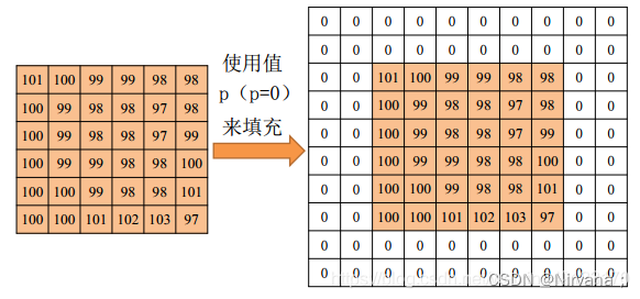
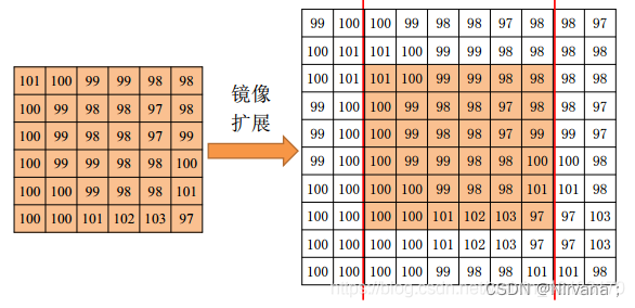
2)symmetric symmetry : The input array value outside the array boundary is obtained by specular reflection of the array along the array boundary 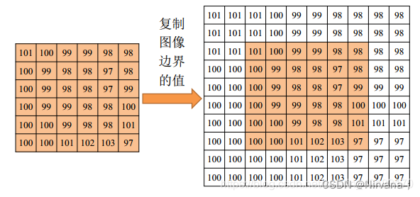
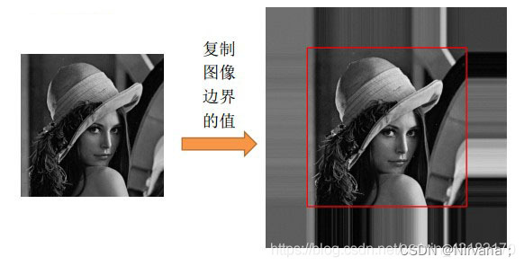
3)replicate Copy : The input array value outside the array boundary is assumed to be equal to the nearest array boundary value 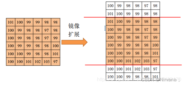 .
.
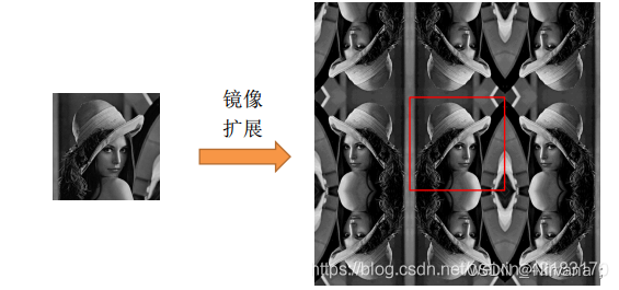
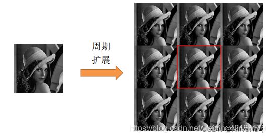
4)circular loop : The input array value outside the array boundary is calculated by implicitly assuming that the input array is periodic .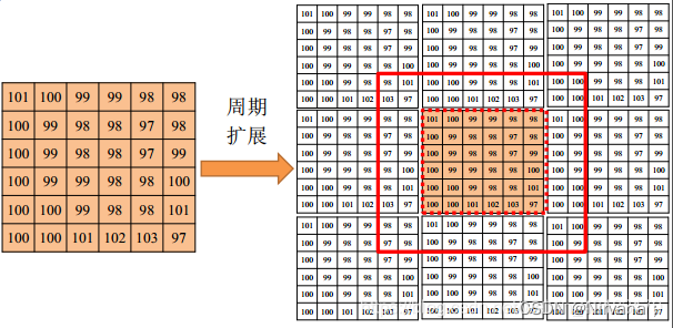
Output Size Output size
same: The output array is the same size as the input array . This is the default behavior when the output size option is not specified .
full: The output array is the result of complete filtering , Therefore, it is larger than the input array .
6. fspecial function
effect : Constructing convolution kernel , It can be done with filter2、conv2 and imfilter In combination with
h = fspecial(type)
h = fspecial('average',hsize)
h = fspecial('disk',radius)
h = fspecial('gaussian',hsize,sigma)
h = fspecial('laplacian',alpha)
h = fspecial('log',hsize,sigma)
h = fspecial('motion',len,theta)
h = fspecial('prewitt')
h = fspecial('sobel')

7. summary
filter2、conv2 Convert the input to double type , The output is double Of , Input is always filled with zero (zero padded), Other boundary supplement options are not supported .
imfilter: Do not convert input to double, Output is only of the same type as input , There are flexible boundary supplement options . It is recommended to use ~
8. Code demonstration
MATLAB Code :
clear;
close all;
clc;

%% fspecial function
value = 5;
h = fspecial('gaussian',[5 5],value);

srcImage = imread('lena.jpg');
srcImage = rgb2gray(srcImage);
srcImage_double = double(srcImage);

%% conv2 function     Default :'full', Only zero can be filled
image_conv2 = conv2(srcImage_double,h);

%% filter2 function    Default :'same', Only zero can be filled
image_filter2 = filter2(h,srcImage_double);

%% imfilter function   Default :'same'
image_imfilter = imfilter(srcImage,h,'replicate');

%%  Display images
figure(1);
subplot(221);imshow(srcImage,[]); title(' Original picture ');
subplot(222);imshow(image_conv2,[]); title('conv2');
subplot(223);imshow(image_filter2,[]); title('filter2');
subplot(224);imshow(image_imfilter,[]); title('imfilter');
design sketch :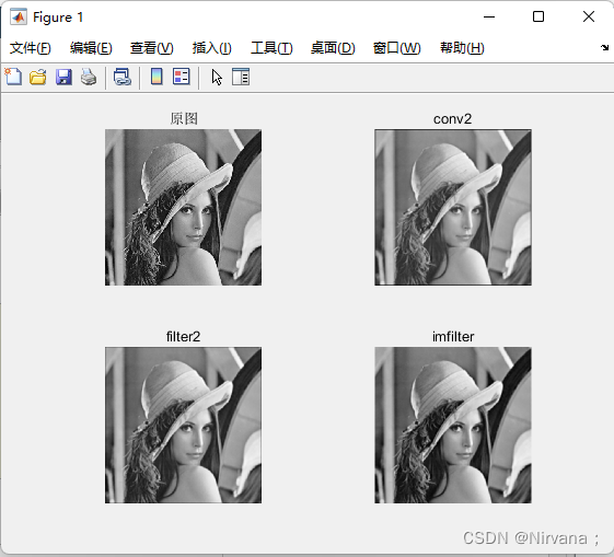
边栏推荐
- 做事的真正意义和目的,真正想得到什么
- .Net之延迟队列
- 软件测试之测试评估
- MySQL5免安装修改
- 2022g3 boiler water treatment examination question simulation examination question bank and simulation examination
- Introduction to reverse debugging PE structure resource table 07/07
- Animation and transition effects
- Deming Lee listed on Shenzhen Stock Exchange: the market value is 3.1 billion, which is the husband and wife of Li Hu and Tian Hua
- 392. 判断子序列
- JVM 内存布局详解,图文并茂,写得太好了!
猜你喜欢

吃透Chisel语言.05.Chisel基础(二)——组合电路与运算符
![[antd step pit] antd form cooperates with input Form The height occupied by item is incorrect](/img/96/379d1692f9d3c05a7af2e938cbc5d7.png)
[antd step pit] antd form cooperates with input Form The height occupied by item is incorrect

DGraph: 大规模动态图数据集
【FAQ】华为帐号服务报错 907135701的常见原因总结和解决方法
Unittest中的TestSuite和TestRunner
安装Mysql

華昊中天沖刺科創板:年虧2.8億擬募資15億 貝達藥業是股東
Mask wearing detection based on yolov1

Huahao Zhongtian rushes to the scientific and Technological Innovation Board: the annual loss is 280million, and it is proposed to raise 1.5 billion. Beida pharmaceutical is a shareholder

2022 hoisting machinery command examination simulation 100 questions simulation examination platform operation
随机推荐
2022G3锅炉水处理考试题模拟考试题库及模拟考试
Interviewer: what is the internal implementation of hash data type in redis?
php 日志调试
常见 content-type对应表
Animation and transition effects
Fs4056 800mA charging IC domestic fast charging power IC
sharding key type not supported
面试拆解:系统上线后Cpu使用率飙升如何排查?
读取 Excel 表数据
Mask wearing detection based on yolov1
The Secretary of Homeland Security warned immigrants "not to embark on a dangerous journey"
基于PaddleX的智能零售柜商品识别
1200. 最小绝对差
Haproxy high availability solution
吃透Chisel语言.09.Chisel项目构建、运行和测试(一)——用sbt构建Chisel项目并运行
好博医疗冲刺科创板:年营收2.6亿 万永钢和沈智群为实控人
吃透Chisel语言.04.Chisel基础(一)——信号类型和常量
博士申请 | 西湖大学学习与推理系统实验室招收博后/博士/研究实习等
Applet live + e-commerce, if you want to be a new retail e-commerce, use it!
Unity Shader学习(三)试着绘制一个圆