Hands on deep learning (IV) -- convolutional neural network CNN

         In the previous section, I learned the implementation of convolution layer and pooling layer of convolution neural network , Strike while the iron is hot and continue to learn the construction of modern Convolutional Neural Networks , Welcome friends to study and communicate together ~

         In order to be able to respond ⽤softmax Regression and multi-layer perceptron , We ⾸ First, put each ⼤ Xiao Wei $28\times 28$ The image is flattened to ⼀ individual 784 Fixation of dimension ⻓ Degree ⼀ Dimension vector , then ⽤ The whole connection layer is for it ⾏ Handle . And now , We have mastered the treatment of convolution ⽅ Law , You can preserve the spatial structure in the image . meanwhile ,⽤ Convolution layer replaces another of the full connection layer ⼀ One advantage is that ： The model is more concise 、 Fewer parameters required .

         There are many detailed introductions and advantages and disadvantages of these networks on the Internet , Here we just introduce the composition and implementation of various convolution Networks . These models include ：

• LeNet. Convolutional neural network, which was first released ⽹ Collaterals ⼀;
• AlexNet. The first ⼀ It's in ⼤ Beat the traditional computer vision model in the scale vision competition ⼤ Type nerve ⽹ Collateral ;
• send ⽤ Repeated block ⽹ Collateral （VGG）. benefit ⽤ Many repetitive nerves ⽹ Collaterals ;
• ⽹ Collateral ⽹ Collateral （NiN）. Repeat make ⽤ Composed of convolution and $1\times 1$ Convolution layer （⽤ To replace the full connection layer ） To build deep ⽹ Collateral ;
• Contain and ⾏ Connected ⽹ Collateral （GoogLeNet）. send ⽤ and ⾏ Connected ⽹ Collateral , Through different windows ⼤ Small convolution layers and the most ⼤ Convergence layer and ⾏ Extract information ;
• residual ⽹ Collateral （ResNet）. Build cross layer data channels through residual blocks , It is the most popular in computer vision ⾏ The architecture of ;
• Dense connections ⽹ Collateral （DenseNet）. Calculating the cost is very ⾼, But it has brought us better results .

---

1 LeNet

1.1 Model structures,

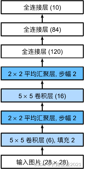
        LeNet（LeNet-5） It consists of two parts ：（1） Convolutional encoder ： It consists of two convolutions ;（2） Full connection layer dense blocks ： It consists of three fully connected layers . The architecture is shown in the following figure ：

LeNet Data flow in . transport ⼊ yes ⼿ Write numbers , Output is 10 The probability of a possible outcome .

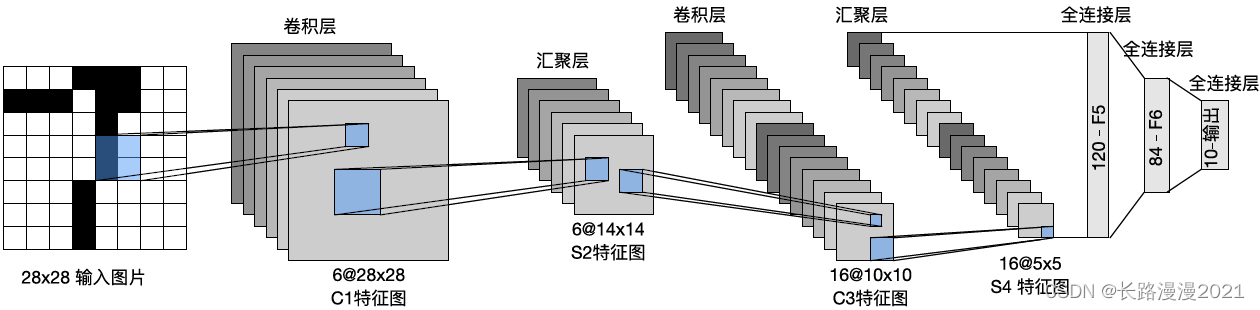
         The basic unit in each convolution block is ⼀ Convolution layers 、⼀ individual sigmoid Activation function and average convergence layer . Please note that , although ReLU And the most ⼤ The convergence layer is more effective , But they are 20 century 90 The age has not yet appeared . Each convolution layer makes ⽤$5\times 5$ Convolution kernels and ⼀ individual sigmoid Activation function . These layers will lose ⼊ Map to multiple ⼆ Dimension feature output , Usually increase the number of channels at the same time . The first ⼀ The convolution layer has 6 Output channels , And the first ⼆ There are three convolution layers 16 Output channels . Every $2\times 2$ Pooling operation （ step 2） The dimension is reduced by spatial down sampling 4 times . The output shape of convolution is determined by batch ⼤ Small 、 The channel number 、⾼ degree 、 Width determination .

         In order to pass the output of convolution block to dense block , We have to flatten each sample in a small batch . in ⾔ And , Lose this four dimension ⼊ Convert to what the full connection layer expects ⼆ Maintenance and transportation ⼊. this ⾥ Of ⼆ Dimension table ⽰ Of the ⼀ Dimension index samples in small batches , The first ⼆ Four dimensions give the average of each sample ⾯ Vector table ⽰.LeNet The dense block of has three full connection layers , There were 120、84 and 10 Outputs . Because we are still holding ⾏ classification , So the output layer 10 The dimension corresponds to the number of final output results .LeNet You only need to instantiate one Sequential Block and connect the required layers together .

import torch
from torch import nn
from d2l import torch as d2l
from torchvision import transforms
from torch.utils.data import DataLoader
from mnist_dataset import FashionMnistDataset   #  Custom dataset import 

#  Model structures, 
LeNet = nn.Sequential(
    nn.Conv2d(1, 6, kernel_size=5, padding=2), nn.Sigmoid(),
    nn.AvgPool2d(kernel_size=2, stride=2),
    nn.Conv2d(6, 16, kernel_size=5), nn.Sigmoid(),
    nn.AvgPool2d(kernel_size=2, stride=2),
    nn.Flatten(),
    nn.Linear(16 * 5 * 5, 120), nn.Sigmoid(),
    nn.Linear(120, 84), nn.Sigmoid(),
    nn.Linear(84, 10))

         The original model is made here ⼀ A little change , Remove the last ⼀ Layer of ⾼ S activation . besides , This ⽹ Collaterals with the original LeNet-5⼀ Cause .

         Next ⾯, We will ⼀ individual ⼤ Xiao Wei $28\times 28$ Single channel （⿊⽩） The image passes through LeNet. Through every ⼀ The shape of the layer printout , We can check the model , To ensure that it operates as we expect ⼀ Cause .

LeNet A simplified version of the

X = torch.rand(size=(1, 1, 28, 28), dtype=torch.float32)
for layer in LeNet:
    X = layer(X)
    print(layer.__class__.__name__, 'output shape: \t', X.shape)

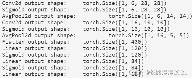
         reminder , In the whole convolution block , And upper ⼀ Stratigraphy ⽐, Every time ⼀ Layer characteristic ⾼ The degree and width are reduced . The first ⼀ A convolution layer makes ⽤2 Pixel fill , To compensate $5\times 5$ The feature reduction caused by convolution kernel . contrary , The first ⼆ The convolution layer is not filled , therefore ⾼ The degree and width are reduced 4 Pixel . As the stack rises , The number of channels is from ⼊ At the time of the 1 individual , Add to ⼀ After a convolution 6 individual , And then to the ⼆ After a convolution 16 individual . meanwhile , Of each convergence layer ⾼ Both degree and width are halved . Last , Each fully connected layer reduces the dimension , Final output ⼀ Output whose dimension matches the number of result classifications .

1.2 model training

         Let's take a look at LeNet stay Fashion-MNIST Performance on dataset .

         Because of the domestic network , Downloading datasets is particularly slow , So use the downloaded local data set , Download datasets online , have access to d2l In the bag load_data_fashion_mnist, as follows ：

batch_size = 256
train_iter, test_iter = d2l.load_data_fashion_mnist(batch_size=batch_size)

         The custom data import is as follows ：

# -*- coding: utf-8 -*-
""" Function Name：mnist_dataset.py Version：0.1 Description： Realization mnsit and Fashion-mnist Import of two datasets  Author：CarpeDiem """
import gzip
import os
import numpy as np
from torch.utils.data import Dataset

class FashionMnistDataset(Dataset):
    """ Reading data 、 Initialization data """
    def __init__(self, folder, data_name, label_name, transform=None):
        (train_set, train_labels) = load_data(folder, data_name, label_name)
        self.train_set = train_set
        self.train_labels = train_labels
        self.transform = transform

    def __getitem__(self, index):
        img, target = self.train_set[index], int(self.train_labels[index])
        if self.transform is not None:
            img = self.transform(img)
        return img, target

    def __len__(self):
        return len(self.train_set)


def load_data(data_folder, data_name, label_name):
    with gzip.open(os.path.join(data_folder, label_name), 'rb') as labpath:
        y_train = np.frombuffer(labpath.read(), np.uint8, offset=8)

    with gzip.open(os.path.join(data_folder, data_name), 'rb') as imgpath:
        x_train = np.frombuffer(imgpath.read(), np.uint8,
                                offset=16).reshape(len(y_train), 28, 28)

    return (x_train, y_train)

#  Dataset import 
batch_size = 256
transform  = transforms.Compose([transforms.ToTensor()])
train_dataset = FashionMnistDataset('../dataset/fashion-mnist', 'train-images-idx3-ubyte.gz', 'train-labels-idx1-ubyte.gz',  transform=transform)
train_loader = DataLoader(train_dataset, shuffle=True, batch_size=batch_size)
test_dataset = FashionMnistDataset('../dataset/fashion-mnist', 't10k-images-idx3-ubyte.gz', 't10k-labels-idx1-ubyte.gz', transform=transform)
test_loader = DataLoader(test_dataset, shuffle=False, batch_size=batch_size)

         Although convolution nerve ⽹ The parameters of the complex are less , But with the depth of the multi-layer perceptron ⽐, Their computational costs are still very ⾼, Because each parameter is involved in more multiplication . This is where ⽤GPU Speed up training . Rewrite here evaluate_accuracy function .

def evaluate_accuracy_gpu(net, data_loader, device=None):
    """ Use GPU Calculate the accuracy of the model on the dataset """
    if isinstance(net, nn.Module):
        net.eval()      #  Set to evaluation mode 
        if not device:
            device = next(iter(net.parameters())).device
    #  The number of correct predictions , Total forecast quantity 
    metric = d2l.Accumulator(2)
    with torch.no_grad():
        for X, y in data_loader:
            if isinstance(X, list):
                X = [x.to(device) for x in X]
            else:
                X = X.to(device)
            y = y.to(device)
            metric.add(d2l.accuracy(net(X), y), y.numel())
    return metric[0] / metric[1]

         In into ⾏ Before forward and backward propagation , We need to put every ⼀ Small batch data is moved to our designated equipment （ for example GPU） On . With full connection layer ⼀ sample , send ⽤ Cross entropy loss function and small batch random gradient descent , The training model is as follows .

def train_ch6(net, train_loader, test_loader, num_epoches, lr, device):
    """ use GPU Training models """
    def init_weights(m):
        if isinstance(m, nn.Linear) or isinstance(m, nn.Conv2d):
            nn.init.xavier_normal_(m.weight)
    net.apply(init_weights)
    print('training on', device)
    net.to(device)
    optimizer = torch.optim.SGD(net.parameters(), lr=lr)
    criterion = nn.CrossEntropyLoss()
    animator = d2l.Animator(xlabel='epoch', xlim=[1, num_epoches], legend=['train loss', 'train acc', 'test acc'])
    timer, num_batches = d2l.Timer(), len(train_loader)
    for epoch in range(num_epoches):
        #  The sum of training losses , The sum of training accuracy , Number of examples 
        metric = d2l.Accumulator(3)
        net.train()
        for iteration, (X, y) in enumerate(train_loader):
            timer.start()
            optimizer.zero_grad()
            X, y = X.to(device), y.to(device)
            y_hat = net(X)
            loss = criterion(y_hat, y)
            loss.backward()
            optimizer.step()
            with torch.no_grad():
                metric.add(loss * X.shape[0], d2l.accuracy(y_hat, y), X.shape[0])
            timer.stop()
            train_loss = metric[0] / metric[2]
            train_acc = metric[1] / metric[2]
            if (iteration + 1) % (num_batches // 5) == 0 or iteration == num_batches - 1:       #  Every time num_batches//5 Calculate the loss and training accuracy every time 
                animator.add(epoch + (iteration + 1) / num_batches, (train_loss, train_acc, None))
        test_acc = evaluate_accuracy_gpu(net, test_loader)      #  After a round of training, calculate the accuracy of prediction 
        animator.add(epoch+1, (None, None, test_acc))
    print(f'loss {
      train_loss:.3f}, train acc {
      train_acc:.3f}, test acc {
      test_acc:.3f}')
    print(f'{
      metric[2] * num_epoches / timer.sum():.1f} examples/sec, on {
      str(device)}')

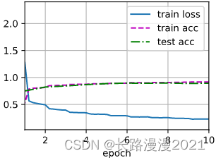
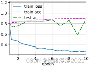
         Next , Training and evaluation LeNet-5 Model .

lr, num_epochs = 0.9, 10
train_ch6(LeNet, train_loader, test_loader,num_epochs, lr, d2l.try_gpu())
# loss 0.465, train acc 0.826, test acc 0.824
# 84969.9 examples/sec, on cuda:0

---

2 AlexNet

        2012 year ,AlexNet Born in the sky . it ⾸ This proves that the learned characteristics can surpass ⼿⼯ Design features . it ⼀ It breaks the current situation of computer vision research .AlexNet send ⽤ 了 8 Layer convolution nerve ⽹ Collateral , And it's very ⼤ Has won the advantage of 2012 year ImageNet Image recognition challenge .

        AlexNet and LeNet The architecture of ⾮ Often similar , As shown below ⽰. Be careful , this ⾥ Provides ⼀ A slightly simplified version AlexNet, It eliminates the need for two small GPU Design features of simultaneous operation .

from LeNet（ Left ） To AlexNet（ Right ）

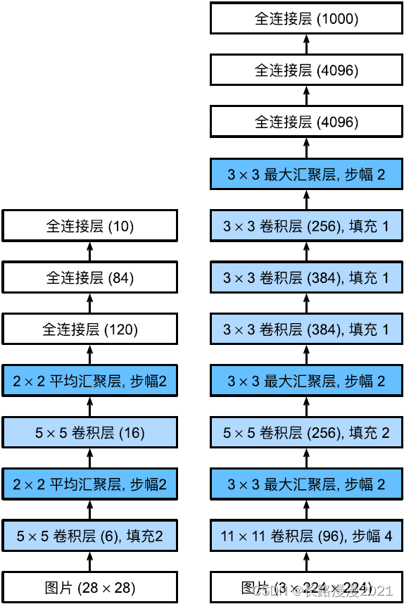
        AlexNet and LeNet Design concept of ⾮ Often similar , But there are also significant differences .⾸ First ,AlexNet⽐ Relatively small LeNet5 Much deeper .AlexNet from ⼋ layers ： Five convolutions 、 Two fully connected hidden layers and ⼀ All connected output layers . secondly ,AlexNet send ⽤ReLU instead of sigmoid As its activation function . Next ⾯, Let's go deep ⼊ Research AlexNet The details of the .

2.1 Model design

         stay AlexNet Of the ⼀ layer , The shape of the convolution window is $11\times 11$. because ImageNet in ⼤ The width and width of most images ⾼⽐MNIST More images 10 More than times , therefore , need ⼀ A change ⼤ Convolution window to capture ⽬ mark . The first ⼆ The convolution window shape in the layer is reduced to $5\times 5$, And then there was $3\times 3$. Besides , In the ⼀ layer 、 The first ⼆ Layer and the fifth layer after the convolution layer , Add ⼊ The window shape is $3\times 3$、 The stride is 2 The most ⼤ Convergence layer . and ,AlexNet Number of convolution channels ⽬ yes LeNet Of 10 times .

         In the end ⼀ There are two fully connected layers behind the convolution layer , There were 4096 Outputs . These two giants ⼤ The full connection layer of has nearly 1GB Model parameters of . Because of the early GPU Limited memory , The original AlexNet Mining ⽤ A dual data flow design , Make each GPU Only responsible for storing and calculating models ⼀ Semiparametric . Fortunately, , Now? GPU Video memory is relatively abundant , So we seldom need to cross GPU Decompose the model （ therefore , our AlexNet The model is here ⽅⾯ And primitive theory ⽂ not quite the same ）.

        AlexNet take sigmoid Change the activation function to a simpler ReLU Activation function .⼀⽅⾯,ReLU The calculation of the activation function is simpler , It doesn't need to be like sigmoid The complex exponentiation of the activation function . another ⼀⽅⾯, When to make ⽤ Different parameter initialization ⽅ Legal time ,ReLU The activation function makes the training model easier . When sigmoid Activate the output of the function ⾮ Often close to 0 or 1 when , The gradient of these areas ⼏ Hu Wei 0, So back propagation ⽆ The law continues to be updated ⼀ Some model parameters . contrary ,ReLU The gradient of the activation function in the positive interval is always 1. therefore , If the model parameters are not initialized correctly ,sigmoid The function may get... In a positive interval ⼏ Hu Wei 0 Gradient of , So that the model ⽆ Get effective training .

        AlexNet adopt dropout Control the model complexity of the whole connection layer , and LeNet Only make ⽤ Weight attenuation .

Alexnet = nn.Sequential(
                        #  this ⾥ send ⽤⼀ individual 11*11 The change of ⼤ window ⼝ To snap objects .
                        #  The stride is 4, To reduce the output ⾼ Degree and width .
                        #  Number of output channels ⽬ far ⼤ On LeNet
                        nn.Conv2d(1, 96, kernel_size=11, stride=4), nn.ReLU(),
                        nn.MaxPool2d(kernel_size=3, stride=2),
                        #  reduce ⼩ Convolution window ⼝, send ⽤ Fill in with 2 To make you lose ⼊ With the output ⾼ And width ⼀ Cause , And increase ⼤ Number of output channels 
                        nn.Conv2d(96, 256, kernel_size=5, padding=2), nn.ReLU(),
                        nn.MaxPool2d(kernel_size=3, stride=2),
                        #  send ⽤ Three consecutive convolution layers and ⼩ Convolution window of ⼝.
                        #  Except for the last convolution layer , The number of output channels goes into ⼀ Step increase .
                        #  After the first two convolutions , The convergence layer is not ⽤ In reducing losses ⼊ Of ⾼ Degree and width 
                        nn.Conv2d(256, 384, kernel_size=3, padding=1), nn.ReLU(),
                        nn.Conv2d(384, 384, kernel_size=3, padding=1), nn.ReLU(),
                        nn.Conv2d(384, 256, kernel_size=3, padding=1), nn.ReLU(),
                        nn.MaxPool2d(kernel_size=3, stride=2),
                        nn.Flatten(),
                        #  this ⾥, The number of outputs of the full connection layer is LeNet Good in ⼏ times . send ⽤dropout Layer to reduce over fitting 
                        nn.Linear(6400, 4096), nn.ReLU(),
                        nn.Dropout(p=0.5),
                        nn.Linear(4096, 4096), nn.ReLU(),
                        nn.Dropout(p=0.5),
                        #  Finally, the output layer . Because of this ⾥ send ⽤Fashion-MNIST, therefore ⽤ The number of categories is 10,⽽⾮ On ⽂ Medium 1000
                        nn.Linear(4096, 10))

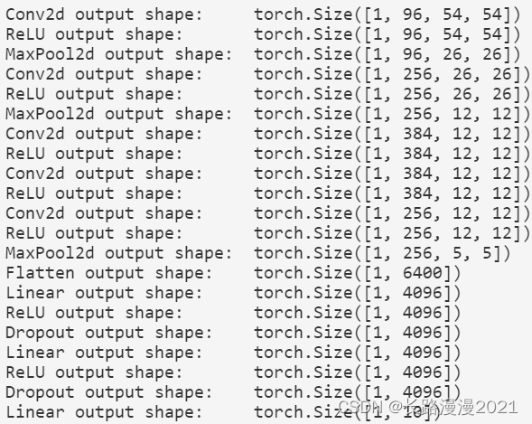
         structure ⼀ individual ⾼ Degree and width are 224 Single channel data of , To observe every ⼀ The shape of the layer output .

X = torch.randn(1, 1, 224, 224)
for layer in Alexnet:
    X = layer(X)
    print(layer.__class__.__name__, 'output shape:\t', X.shape)

2.2 Reading data sets

         Although Ben ⽂ in AlexNet Is in ImageNet progresses ⾏ Trained , But we're here ⾥ send ⽤ Yes. Fashion-MNIST Data sets . Because even in modern times GPU On , Training ImageNet Model , At the same time, it may take hours or days to converge . take AlexNet Directly respond to ⽤ On Fashion-MNIST Of ⼀ The problem is ,Fashion-MNIST The resolution of the image （$28\times 28$ Pixels ） lower than ImageNet Images . To solve this problem , We add them to $224\times 224$（ Generally speaking, this is not ⼀ A wise approach , But we're here ⾥ This is done in order to effectively make ⽤AlexNet framework ）.

#  Dataset import 
batch_size = 256
resize = 224
transform  = transforms.Compose([transforms.ToTensor(), transforms.Resize(resize)])
train_dataset = FashionMnistDataset('../dataset/fashion-mnist', 'train-images-idx3-ubyte.gz', 'train-labels-idx1-ubyte.gz',  transform=transform)
train_loader = DataLoader(train_dataset, shuffle=True, batch_size=batch_size)
test_dataset = FashionMnistDataset('../dataset/fashion-mnist', 't10k-images-idx3-ubyte.gz', 't10k-labels-idx1-ubyte.gz', transform=transform)
test_loader = DataLoader(test_dataset, shuffle=False, batch_size=batch_size)

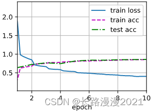
2.3 Training AlexNet

         With the last section of LeNet phase ⽐, this ⾥ The main change is to make ⽤ Lower learning rate training , This is because ⽹ The collaterals are deeper and more ⼴、 The image resolution is higher ⾼, Train convolution nerve ⽹ Collaterals are more expensive .

lr, num_epochs = 0.01, 10
d2l.train_ch6(Alexnet, train_loader, test_loader, num_epochs, lr, d2l.try_gpu())
# loss 0.402, train acc 0.853, test acc 0.859
# 3433.1 examples/sec on cuda:0

---

3 VGG

3.1 VGG block

         Classical convolutional nerve ⽹ The basic component of collaterals is lower ⾯ This sequence of ：1. Convolution layer with filling to maintain resolution ;1. ⾮ Linear activation function , Such as ReLU;1. Convergence layer , Like the most ⼤ Convergence layer .

         and ⼀ individual VGG Block is similar to it , from ⼀ Series convolution layer composition , after ⾯ Plus ⽤ The most..., sampled in space ⼤ Convergence layer . In the initial VGG On ⽂Simonyan & Zisserman, 2014 in , The author made ⽤ With $3\times 3$ Convolution kernel 、 Fill in with 1（ keep ⾼ Degree and width ） The convolution of layer , And with $2\times 2$ Convergence window 、 The stride is 2（ The resolution after each block is halved ） The most ⼤ Convergence layer . Under ⾯ In the code of , Defined ⼀ One is called vgg_block The function of ⼀ individual VGG block . This function has three arguments , Corresponding to the number of convolution layers num_convs、 transport ⼊ The number of channels in_channels And the number of output channels out_channels.

def vgg_block(num_convs, in_channels, out_channels):
    layers = []
    for _ in range(num_convs):
        layers.append(nn.Conv2d(in_channels, out_channels, kernel_size=3, padding=1))
        layers.append(nn.ReLU())
        in_channels = out_channels
    layers.append(nn.MaxPool2d(kernel_size=2, stride=2))
    return nn.Sequential(*layers)

3.2 VGG The Internet

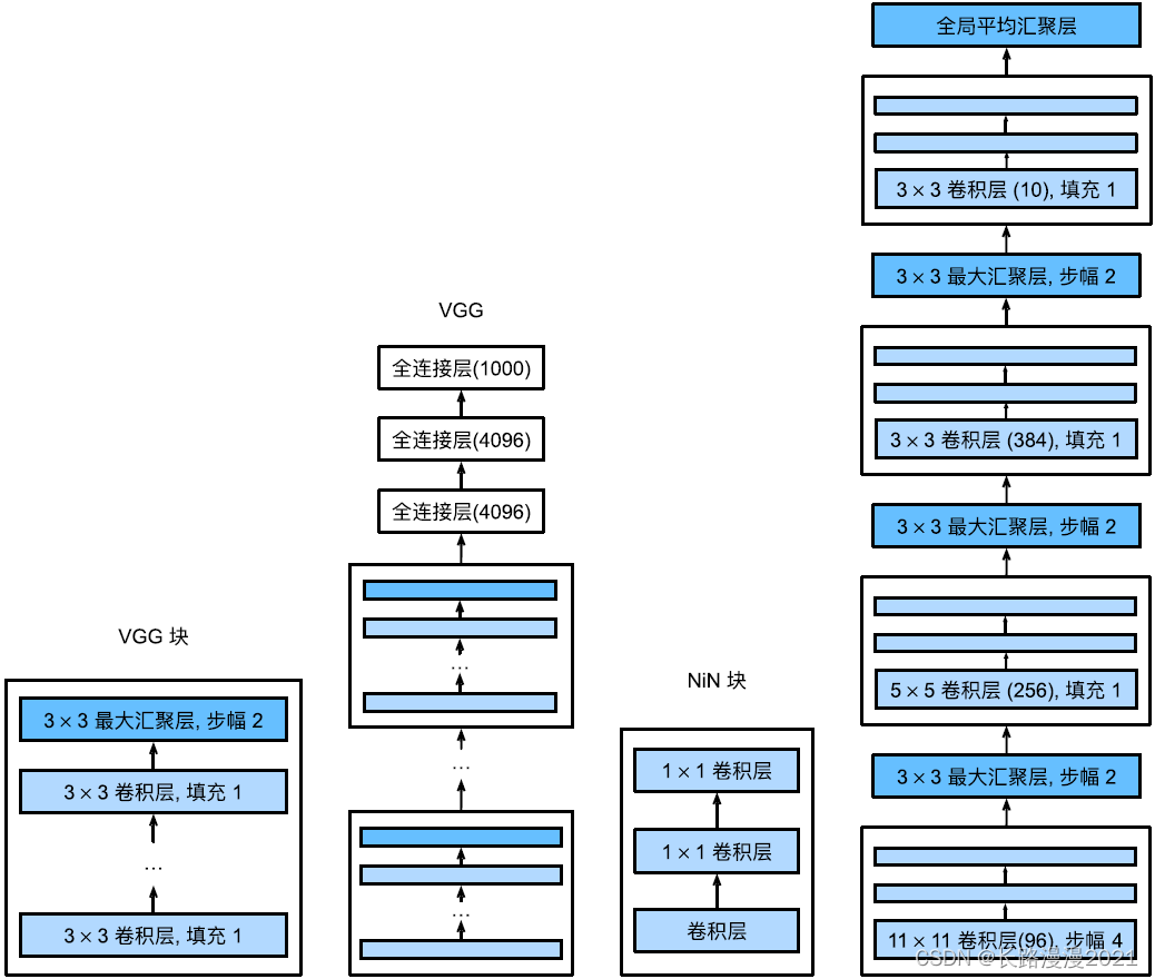
         And AlexNet、LeNet⼀ sample ,VGG⽹ Collaterals can be divided into two parts ： The first ⼀ The part is mainly composed of convolution layer and convergence layer , The first ⼆ Part consists of the whole connection layer . The network structure is shown in the figure below .

from AlexNet To VGG, They are all block designs in essence

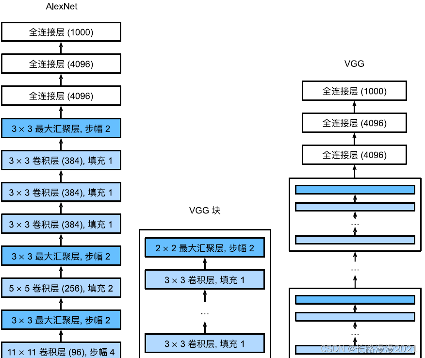
        VGG nerve ⽹ The network connects the ⼏ individual VGG block （ stay vgg_block Function ）. There are super parametric variables conv_arch. This variable specifies each VGG block ⾥ Number of convolution layers and output channels . The fully connected module is connected with AlexNet The same in .

         original VGG⽹ Collaterals 5 Convolution blocks , The first two blocks each have ⼀ Convolution layers , The last three blocks each contain two convolution layers . The first ⼀ There are two modules 64 Output channels , Each subsequent module doubles the number of output channels , Until the number reaches 512. Because of the ⽹ Collateral envoy ⽤8 Convolutions and 3 All connection layers , So it's often called VGG-11. Next ⾯ The code of VGG-11. It can be done by conv_arch Hold on to ⾏for Loop to simply implement .

def vgg(conv_arch):
    conv_blks = []
    in_channels = 1
    for (num_convs, out_channels) in conv_arch:
        conv_blks.append(vgg_block(num_convs, in_channels, out_channels))
        in_channels = out_channels
    
    return nn.Sequential(
        *conv_blks, nn.Flatten(),
        nn.Linear(out_channels * 7 * 7, 4096), nn.ReLU(), nn.Dropout(0.5),
        nn.Linear(4096, 4096), nn.ReLU(), nn.Dropout(0.5), 
        nn.Linear(4096, 10))

conv_arch = ((1, 64), (1, 128), (2, 256), (2, 512), (2, 512))
net = vgg(conv_arch)

Next , structure ⼀ individual ⾼ Degree and width are 224 Single channel data sample , To observe the shape of the output of each layer .

X = torch.rand(size=(1, 1, 224, 224))
for blk in net:
    X = blk(X)
    print(blk.__class__.__name__, 'output shape:\t', X.shape)

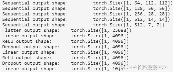
         You can find , In each block ⾼ Half the degree and width , Final ⾼ Degree and width are 7. Finally, flatten the table ⽰, send ⼊ Full connection layer processing .

3.3 Training models

         because VGG-11⽐AlexNet The amount of calculation is more ⼤, So we built ⼀ Less channels ⽹ Collateral ,⾜ enough ⽤ In training Fashion-MNIST Data sets .

ratio = 4
small_conv_arch = [(pair[0], pair[1] // ratio) for pair in conv_arch]
net = vgg(small_conv_arch)

         The model training process is the same as that in the previous section AlexNet similar .

lr, num_epochs = 0.05, 10
d2l.train_ch6(net, train_loader, test_loader, num_epochs, lr, d2l.try_gpu())
# loss 0.228, train acc 0.917, test acc 0.894
# 1851.7 examples/sec on cuda:0

---

4 NiN

        LeNet、AlexNet and VGG There are ⼀ Common design patterns ： adopt ⼀ A series of convolution layers and convergence layers are used to extract spatial structure features ; Then, through the characterization of the features of the full connection layer ⾏ Handle .AlexNet and VGG Yes LeNet The improvement of mainly lies in how to expand ⼤ And deepen these two modules . perhaps , It is conceivable to make ⽤ Fully connected layer . However , If so ⽤ A full connection layer , May completely abandon the spatial structure of representation .⽹ Collateral ⽹ Collateral （NiN） Provides ⼀ individual ⾮ Often simple solution ⽅ case ： Make ⽤ Multilayer perceptron .

4.1 NiN block

        NiN The idea is at each pixel position （ For each ⾼ Degree and width ） Should be ⽤⼀ All connection layers . If we connect weights to each spatial location , We can think of it as $1\times 1$ Convolution layer , Or as unique in each pixel position ⽴ do ⽤ The full connection layer of . From the other side ⼀ individual ⻆ To see , That is, each pixel in the spatial dimension is regarded as a single sample , Consider channel dimensions as different characteristics （feature）.

         The following figure illustrates VGG and NiN And the main architectural differences between their blocks .NiN Block with ⼀ Start with an ordinary convolution , after ⾯ Are the two $1\times 1$ The convolution of layer . these two items. $1\times 1$ The convolution layer acts as a band ReLU Activate the pixel by pixel full connection layer of the function . The first ⼀ The convolution window shape of a layer is usually determined by ⽤⼾ Set up . The subsequent convolution window shape is fixed to $1\times 1$.

Yes ⽐VGG and NiN And the main architectural differences between their blocks

def nin_block(in_channels, out_channels, kernel_size, strides, padding):
    return nn.Sequential(
        nn.Conv2d(in_channels, out_channels, kernel_size, strides, padding),
        nn.ReLU(),
        nn.Conv2d(out_channels, out_channels, kernel_size=1), nn.ReLU(),
        nn.Conv2d(out_channels, out_channels, kernel_size=1), nn.ReLU())

4.2 NiN Model

        NiN send ⽤ The window shape is $11\times 11$、$5\times 5$ and $3\times 3$ The convolution of layer , The number of output channels is the same as AlexNet The same in . Every NiN There is... Behind the block ⼀ The most ⼤ Convergence layer , The shape of the convergence window is $3\times 3$, The stride is 2.

        NiN and AlexNet Between ⼀ One notable difference is NiN The full connection layer has been completely eliminated . contrary ,NiN send ⽤⼀ individual NiN block , The number of output channels is equal to the number of label categories . At last ⼀ Global average convergence layer （global average pooling layer）,⽣ become ⼀ Multiple logic vectors （logits）.NiN The design of the ⼀ One advantage is , It significantly reduces the number of parameters required by the model . However , In practice , This design sometimes increases the time of training the model .

net = nn.Sequential(
    nin_block(1, 96, kernel_size=11, strides=4, padding=0),
    nn.MaxPool2d(3, stride=2),
    nin_block(96, 256, kernel_size=5, strides=1, padding=2),
    nn.MaxPool2d(3, stride=2),
    nin_block(256, 384, kernel_size=3, strides=1, padding=1),
    nn.MaxPool2d(3, stride=2),
    nn.Dropout(0.5),
    nin_block(384, 10, kernel_size=3, strides=1, padding=1),
    nn.AdaptiveAvgPool2d((1, 1)),
    #  Convert the four-dimensional output to ⼆ Output of dimension , Its shape is ( Batch ⼤⼩,10)
    nn.Flatten())

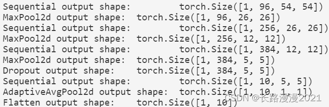
         establish ⼀ Data samples to see the output shape of each block .

X = torch.rand(size=(1, 1, 224, 224))
for layer in net:
    X = layer(X)
    print(layer.__class__.__name__, 'output shape:\t', X.shape)

4.3 Training models

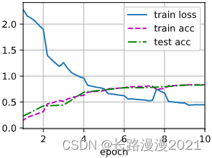
         And before ⼀ sample , send ⽤Fashion-MNIST To train the model . Training NiN And training AlexNet、VGG Time similarity .

lr, num_epochs = 0.1, 10
d2l.train_ch6(net, train_loader, test_loader, num_epochs, lr, d2l.try_gpu())
# loss 0.448, train acc 0.833, test acc 0.827
# 2613.3 examples/sec on cuda:0

---

5 GoogLeNet

         stay GoogLeNet in , The basic convolution block is called Inception block （Inception block）. It's probably named after the movie 《 Inception 》（Inception）, Because in the movie ⼀ Sentence “ We need to go deeper ”（“We need to go deeper”）.

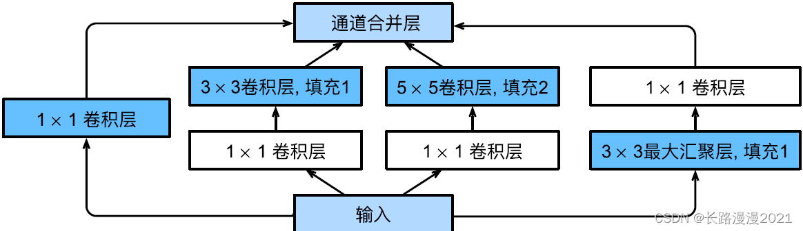
5.1 Inception block

         As shown in the figure below ,Inception The block consists of four and ⾏ Path composition . The first three paths make ⽤ window ⼤ Xiao Wei $1\times 1$、$3\times 3$ and $5\times 5$ The convolution of layer , From different spaces ⼤ Extract information from small . The two paths in the middle are losing ⼊ Hold on to ⾏$1\times 1$ Convolution , To reduce the number of channels , So as to reduce the complexity of the model . The fourth path makes ⽤$3\times 3$ most ⼤ Convergence layer , Then make ⽤$1\times 1$ Convolution layer to change the number of channels . All four paths make ⽤ Fill properly to make it lose ⼊ With the output ⾼ And width ⼀ Cause , Finally, we link the output of each line in the channel dimension , And constitute Inception Block output . stay Inception In block , Usually, the super parameter to be adjusted is the number of output channels per layer .

Inception The architecture of the block

from torch.nn import functional as F
class Inception(nn.Module):
    # c1--c4 Is the number of output channels per path 
    def __init__(self, in_channels, c1, c2, c3, c4, **kwargs):
        super(Inception, self).__init__(**kwargs)
        #  line 1, single 1×1 Convolution layer 
        self.p1_1 = nn.Conv2d(in_channels, c1, kernel_size=1)
        #  line 2,1x1 Convolution layer followed by 3x3 Convolution layer 
        self.p2_1 = nn.Conv2d(in_channels, c2[0], kernel_size=1)
        self.p2_2 = nn.Conv2d(c2[0], c2[1], kernel_size=3, padding=1)
        #  line 3,1x1 Convolution layer followed by 5x5 Convolution layer 
        self.p3_1 = nn.Conv2d(in_channels, c3[0], kernel_size=1)
        self.p3_2 = nn.Conv2d(c3[0], c3[1], kernel_size=5, padding=2)
        #  line 4,3x3 most ⼤ The convergence layer is followed by 1x1 Convolution layer 
        self.p4_1 = nn.MaxPool2d(kernel_size=3, stride=1, padding=1)
        self.p4_2 = nn.Conv2d(in_channels, c4, kernel_size=1)
    
    def forward(self, x):
        p1 = F.relu(self.p1_1(x))
        p2 = F.relu(self.p2_2(F.relu(self.p2_1(x))))
        p3 = F.relu(self.p3_2(F.relu(self.p3_1(x))))
        p4 = F.relu(self.p4_2(self.p4_1(x)))
        #  Link the output in the channel dimension 
        return torch.cat((p1, p2, p3, p4), dim=1)

         So why GoogLeNet This ⽹ Collaterals are so effective ？⾸ Let's think about it first ⼀ Lower filter （filter） The combination of , They can ⽤ Various filter rulers ⼨ Explore images , It means different ⼤ Small filters can effectively identify different ranges of image details . meanwhile , We can assign different numbers of parameters to different filters .

5.2 GoogLeNet Model

        GoogLeNet⼀ Make... Together ⽤9 individual Inception Stack of blocks and global average convergence layer ⽣ Become its estimated value .Inception The most ⼤ The aggregation layer can reduce the dimension . The first ⼀ Modules are similar to AlexNet and LeNet,Inception Combination of blocks from VGG Inherit , The global average convergence layer avoids making ⽤ Fully connected layer . The network structure is shown in the figure below .

GoogLeNet framework

         By ⼀ Realization GoogLeNet Each module of . The first ⼀ Two modules make ⽤64 Channels 、$7\times 7$ Convolution layer .

b1 = nn.Sequential(nn.Conv2d(1, 64, kernel_size=7, stride=2, padding=3),
                    nn.ReLU(),
                    nn.MaxPool2d(kernel_size=3, stride=2, padding=1))

         The first ⼆ Two modules make ⽤ Two layers of convolution ： The first ⼀ A convolution layer is 64 Channels 、$1\times 1$ Convolution layer ; The first ⼆ A convolution layer makes ⽤ Tripled the number of channels $3\times 3$ Convolution layer . This corresponds to Inception The... In the block ⼆ Paths .

b2 = nn.Sequential(nn.Conv2d(64, 64, kernel_size=1),
                    nn.ReLU(),
                    nn.Conv2d(64, 192, kernel_size=3, padding=1),
                    nn.ReLU(),
                    nn.MaxPool2d(kernel_size=3, stride=2, padding=1))

         The third module connects two complete modules in series Inception block . The first ⼀ individual Inception The number of output channels of the block is 64 + 128 + 32 + 32 = 256, Number of output channels between the four paths ⽐ by 64 : 128 : 32 : 32 = 2 : 4 : 1 : 1. The first ⼆ The first and third paths ⾸ Lose first ⼊ The number of channels is reduced to 96/192 = 1/2 and 16/192 = 1/12, Then connect the second ⼆ Convolution layers . The first ⼆ individual Inception Increase the number of output blocks to 128 + 192 + 96 + 64 = 480, Number of output channels between the four paths ⽐ by 128 : 192 : 96 : 64 = 4 : 6 : 3 : 2. The first ⼆ And the third path ⾸ Lose first ⼊ The number of channels is reduced to 128/256 = 1/2 and 32/256 = 1/8.

b3 = nn.Sequential(Inception(192, 64, (96, 128), (16, 32), 32),
                   Inception(256, 128, (128, 192), (32, 96), 64),
                   nn.MaxPool2d(kernel_size=3, stride=2, padding=1))

         The fourth module is more complex , It's connected in series 5 individual Inception block , The number of output channels is 192+208+48+64 = 512、160+224+64 + 64 = 512、128 + 256 + 64 + 64 = 512、112 + 288 + 64 + 64 = 528 and 256 + 320 + 128 + 128 = 832. The channel number allocation of these paths is similar to that in the third module ,⾸ First, including 3×3 In the convolution layer ⼆ The maximum number of output channels per path , Secondly, it only contains 1×1 In the convolution layer ⼀ Paths , And then there's 5×5 The third path of convolution layer and containing 3×3 most ⼤ The fourth path of the convergence layer . Among them the first ⼆、 The third path will first press ⽐ For example, reduce the number of channels . these ⽐ For example, in each Inception The blocks are all slightly different .

b4 = nn.Sequential(Inception(480, 192, (96, 208), (16, 48), 64),
                   Inception(512, 160, (112, 224), (24, 64), 64),
                   Inception(512, 128, (128, 256), (24, 64), 64),
                   Inception(512, 112, (144, 288), (32, 64), 64),
                   Inception(528, 256, (160, 320), (32, 128), 128),
                   nn.MaxPool2d(kernel_size=3, stride=2, padding=1))

         The fifth module contains output channels with a number of 256 + 320 + 128 + 128 = 832 and 384 + 384 + 128 + 128 = 1024 Of the two Inception block . The allocation idea of the number of channels per path is the same as the third one 、 In the fourth module ⼀ Cause , It's just different in terms of specific values . It should be noted that , After the fifth module ⾯ Follow the output layer , This module is the same as NiN⼀ How to make ⽤ Global average convergence layer , The of each channel ⾼ And width becomes 1. The output will finally become us ⼆ Dimension group , Then put on ⼀ A full connection layer whose output number is the number of label categories .

b5 = nn.Sequential(Inception(832, 256, (160, 320), (32, 128), 128),
                   Inception(832, 384, (192, 384), (48, 128), 128),
                   nn.AdaptiveAvgPool2d((1, 1)),
                   nn.Flatten())
net = nn.Sequential(b1, b2, b3, b4, b5, nn.Linear(1024, 10))       

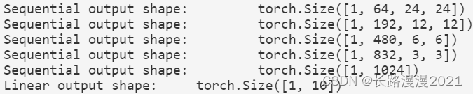
        GoogLeNet The calculation of the model is complicated , And not as good as VGG That makes it easy to change the number of channels . In order to make Fashion-MNIST The training is short and vigorous , We will lose ⼊ Of ⾼ And kuancong 224 drop to 96, This simplifies the calculation . Next ⾯ Play ⽰ The shape of the output of each module changes .

X = torch.rand(size=(1, 1, 96, 96))
for layer in net:
    X = layer(X)
    print(layer.__class__.__name__, 'output shape:\t', X.shape)

5.3 Training models

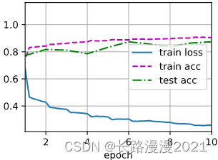
         And before ⼀ sample , We make ⽤Fashion-MNIST Data sets to train our model . Before training , We're going to figure ⽚ Convert to $96\times 96$ The resolution of the .

#  Dataset import , And change the size 
batch_size = 128
resize = 96
transform  = transforms.Compose([transforms.ToTensor(), transforms.Resize(resize)])
train_dataset = FashionMnistDataset('../dataset/fashion-mnist', 'train-images-idx3-ubyte.gz', 'train-labels-idx1-ubyte.gz',  transform=transform)
train_loader = DataLoader(train_dataset, shuffle=True, batch_size=batch_size)
test_dataset = FashionMnistDataset('../dataset/fashion-mnist', 't10k-images-idx3-ubyte.gz', 't10k-labels-idx1-ubyte.gz', transform=transform)
test_loader = DataLoader(test_dataset, shuffle=False, batch_size=batch_size)

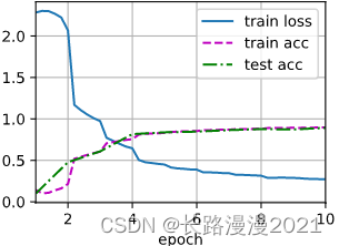
lr, num_epochs = 0.1, 10
d2l.train_ch6(net, train_loader, test_loader, num_epochs, lr, d2l.try_gpu())
# loss 0.274, train acc 0.896, test acc 0.893
# 720.0 examples/sec on cuda:0

---

6 Batch normalization

         Train deep nerves ⽹ Luo is ⼗ Divide difficult , Especially in a short time, it makes them converge more quickly ⼿. In this section , Will introduce Batch normalization （batch normalization）, This is a ⼀ Seed flow ⾏ And effective technology , Sustainable acceleration ⽹ The convergence rate of the complex .

         Batch standardization should ⽤ Apply to a single optional layer （ You can also respond to ⽤ To all layers ）, The principle is as follows ： In each training iteration ,⾸ First normalize the input ⼊, That is, by subtracting its mean and dividing it by its standard deviation , Both of them are based on the current small batch processing . Next , Should be ⽤⽐ Example coefficients and ⽐ Example offset . Because of this standardization based on batch Statistics , The name of batch standardization .

         Please note that , If we try to make ⽤⼤ Xiao Wei 1 Small quantities of should be ⽤ Batch normalization , We will ⽆ I can't find anything . This is because after subtracting the mean , Each hidden cell will be 0. therefore , Only make ⽤⾜ enough ⼤ A small batch of , Batch normalize this ⽅ Law is effective and stable . Please note that , In response to ⽤ When batch normalization , Batch ⼤ Small choices may ⽐ It is more important when there is no batch standardization .

         In form ,⽤$x\text{x}x\in \mathcal{B}$ surface ⽰⼀ Come on ⾃ Small batch $\mathcal{B}$ The loss of ⼊, Batch normalization BN Convert... According to the following expression $x\text{x}x$：
$$\mathrm{BN}(\mathbf{x})=\gamma \odot \frac{\mathbf{x}-{\hat{\mathbf{\mu }}}_{\mathcal{B}}}{{\hat{\sigma }}_{\mathcal{B}}}+\beta$$

         In style ,${\hat{\mathbf{\mu }}}_{\mathcal{B}}$ That's the sample mean ,${\hat{\sigma }}_{\mathcal{B}}$ It's a small batch $\mathcal{B}$ The sample standard deviation of . Should be ⽤ After standardization ,⽣ The average value of the small batch is 0 And units ⽅ The difference is 1. Because the unit ⽅ Bad （ And others ⼀ Some magic numbers ） yes ⼀ An arbitrary choice , So we usually include stretch parameters （scale）$\gamma$ And offset parameters （shift）$\beta$, Their shape is similar to $x\text{x}x$ identical . Please note that ,$\gamma$ and $\beta$ Is required with other model parameters ⼀ Start learning parameters . Because in the process of training , The change range of the middle layer should not be too drastic , And batch standardization will be every ⼀ The layer is actively centered , And readjust them to the given average value and ⼤ Small （ adopt ${\hat{\mathbf{\mu }}}_{\mathcal{B}}$ and ${\hat{\sigma }}_{\mathcal{B}}$）.

         Following calculation ${\hat{\mathbf{\mu }}}_{\mathcal{B}}$ and ${\hat{\sigma }}_{\mathcal{B}}$, As shown below ：
$$\begin{gathered} {\hat{\mathbf{\mu }}}_{\mathcal{B}}=\frac{1}{|\mathcal{B}|}\sum _{x\text{x}x\in \mathcal{B}}x\text{x}x \\ {\hat{\sigma }}_{\mathcal{B}}^2=\frac{1}{|\mathcal{B}|}\sum _{x\text{x}x\in \mathcal{B}}(x\text{x}x-{\hat{\mathbf{\mu }}}_{\mathcal{B}}{)}^2+ϵ \end{gathered}$$

         Please note that , We are ⽅ Add... To the difference estimate ⼀ A small constant $ϵ>0$, To make sure we never try to divide by zero , Even in experience ⽅ The same is true when the difference estimate may disappear .

6.1 Batch normalization layer

1. Fully connected layer

         Usually , We put the batch normalization layer between the affine transformation and the activation function in the full connection layer . Set the transmission line of the whole connection layer ⼊ by $u\text{u}u$, The weight parameter and offset parameter are respectively $W\text{W}W$ and $b\text{b}b$, The activation function is $\varphi$, The operator of batch normalization is BN. that , send ⽤ The calculation details of the output of the batch normalized full connection layer are as follows ：
$$\mathbf{h}=\varphi (\mathrm{BN}(\mathbf{W}\mathbf{x}+\mathbf{b}))$$

2. Convolution layer

         For the convolution layer , We can after the accretion layer and ⾮ The linear activation function should be preceded by ⽤ Batch normalization . When convolution has multiple output channels , We need to control these channels “ Every ” Output execution ⾏ Batch normalization , Every channel has ⾃⼰ The stretch of （scale） And offset （shift） Parameters , Both parameters are scalars . Suppose our micro batch contains m individual ⽰ example , And for each channel , The output of convolution has ⾼ degree p Width and width q. So for the convolution layer , We are at the end of each output channel $m\times p\times q$ Execute simultaneously on two elements ⾏ Each batch is normalized . therefore , In calculating the average and ⽅ Differential time , All our space values will be collected , Then... In a given channel ⽤ The same mean and ⽅ Bad , In order to enter the value at each spatial position ⾏ Normalization .

3. Batch normalization in the prediction process

         Batch standardization in training mode and prediction mode ⾏ Is usually different .⾸ First , Will train the good model ⽤ When predicting , It is no longer necessary to estimate the noise in the sample mean and the production of each small batch on the micro batch ⽣ The sample of ⽅ The poor . secondly , for example , We may need to make ⽤ Our model is sample by sample ⾏ forecast .⼀ Species often ⽤ Of ⽅ The method is to estimate the sample mean sum of the whole training data set by moving average ⽅ Bad , And make ⽤ They get a definite output .

6.2 From zero

         From scratch ⼀ A batch normalization layer with tensor .

def batch_norm(X, gamma, beta, moving_mean, moving_var, eps, momentum):
    #  adopt is_grad_enabled To determine whether the current mode is training mode or prediction mode 
    if not torch.is_grad_enabled():
        #  If it is in prediction mode , Direct use ⽤ Pass on ⼊ The sum of the mean values obtained from the moving average of ⽅ Bad 
        X_hat = (X - moving_mean) / torch.sqrt(moving_var + eps)
    else:
        assert len(X.shape) in (2, 4)
        if len(X.shape) == 2:
            #  Using full connection , Calculate the mean and variance on the characteristic dimension 
            mean = X.mean(dim=0)
            var = ((X - mean) ** 2).mean(dim=0)
        else:
            #  send ⽤⼆ The condition of dimensional convolution , Calculate the channel dimension （axis=1） The mean and ⽅ Bad .
            #  this ⾥ We need to keep X Shape for later ⾯ You can do it ⼴ Broadcast operation 
            mean = X.mean(dim=(0, 2, 3), keepdim=True)
            var = ((X - mean) ** 2).mean(dim=(0, 2, 3), keepdim=True)
        #  In training mode ,⽤ The current average and ⽅ Poor standardization 
        X_hat = (X - mean) / torch.sqrt(var + eps)
        #  Update the mean and variance of the moving average 
        moving_mean = momentum * moving_mean + (1.0 - momentum) * mean
        moving_var = momentum * moving_var + (1.0 - momentum) * var
    Y = gamma * X_hat + beta #  Zoom and shift 
    return Y, moving_mean.data, moving_var.data

         Now you can create ⼀ It's the right one BatchNorm Layers . This layer will maintain appropriate parameters ： The tensile gamma And offset beta, These two parameters will be updated during the training . Besides , Our layer will save the mean and ⽅ Poor moving average , In order to make ⽤.

class BatchNorm(nn.Module):
    # num_features： The number of outputs of the fully connected layer or the number of output channels of the convolution layer .
    # num_dims：2 surface ⽰ Fully connected layer ,4 surface ⽰ Convolution layer 
    def __init__(self, num_features, num_dims):
        super().__init__()
        if num_dims == 2:
            shape = (1, num_features)
        else:
            shape = (1, num_features, 1, 1)
        #  Stretch and offset parameters involved in gradient sum iteration , Initialize into 1 and 0
        self.gamma = nn.Parameter(torch.ones(shape))
        self.beta = nn.Parameter(torch.zeros(shape))
        # ⾮ The variables of model parameters are initialized to 0 and 1
        self.moving_mean = torch.zeros(shape)
        self.moving_var = torch.ones(shape)

    def forward(self, X):
        #  If X Not in memory , take moving_mean and moving_var
        #  Copied to the X On the video memory 
        if self.moving_mean.device != X.device:
            self.moving_mean = self.moving_mean.to(X.device)
            self.moving_var = self.moving_var.to(X.device)
        #  Save the updated moving_mean and moving_var
        Y, self.moving_mean, self.moving_var = batch_norm(X, self.gamma, self.beta, self.moving_mean, self.moving_var, eps=1e-5, momentum=0.9)
        return Y

6.3 send ⽤ Batch normalization layer LeNet

         Next ⾯ We will BatchNorm Should be ⽤ On LeNet Model .

net = nn.Sequential(
    nn.Conv2d(1, 6, kernel_size=5), BatchNorm(6, num_dims=4), nn.Sigmoid(),
    nn.AvgPool2d(kernel_size=2, stride=2),
    nn.Conv2d(6, 16, kernel_size=5), BatchNorm(16, num_dims=4), nn.Sigmoid(),
    nn.AvgPool2d(kernel_size=2, stride=2), nn.Flatten(),
    nn.Linear(16*4*4, 120), BatchNorm(120, num_dims=2), nn.Sigmoid(),
    nn.Linear(120, 84), BatchNorm(84, num_dims=2), nn.Sigmoid(), 
    nn.Linear(84, 10))

         And before ⼀ sample , We will be in Fashion-MNIST Training on data sets ⽹ Collateral . This code is similar to our first ⼀ Time training LeNet（ Section 1 ） when ⼏ Almost exactly the same , The main difference is the learning rate ⼤ Much more .

lr, num_epochs = 1.0, 10
d2l.train_ch6(net, train_loader, test_loader, num_epochs, lr, d2l.try_gpu())
# loss 0.260, train acc 0.905, test acc 0.874
# 29144.9 examples/sec on cuda:0

         Let's take a look at the first ⼀ Tensile parameters learned from batch normalized layers gamma And offset parameters beta.

net[1].gamma.reshape((-1,)), net[1].beta.reshape((-1,))

6.4 Concise implementation

         You can make ⽤ Defined in the deep learning framework BatchNorm.

net = nn.Sequential(
    nn.Conv2d(1, 6, kernel_size=5), nn.BatchNorm2d(6), nn.Sigmoid(),
    nn.AvgPool2d(kernel_size=2, stride=2),
    nn.Conv2d(6, 16, kernel_size=5), nn.BatchNorm2d(16), nn.Sigmoid(),
    nn.AvgPool2d(kernel_size=2, stride=2), nn.Flatten(),
    nn.Linear(16*4*4, 120), nn.BatchNorm1d(120), nn.Sigmoid(),
    nn.Linear(120, 84), nn.BatchNorm1d(84), nn.Sigmoid(), 
    nn.Linear(84, 10))

lr, num_epochs = 1.0, 10
d2l.train_ch6(net, train_loader, test_loader, num_epochs, lr, d2l.try_gpu())
# loss 0.267, train acc 0.901, test acc 0.883
# 53287.4 examples/sec on cuda:0

         Here we make ⽤ Train the model with the same super parameters . Please note that , Usually ⾼ level API Variant transportation ⾏ Much faster , Because its code has been compiled as C++ or CUDA, And ours ⾃ The definition code is defined by Python Realization .

---

7 ResNet

7.1 Residual block

         Focus on nerves ⽹ Collateral part ： As shown below ⽰, Let's say our original lost ⼊ by $x\text{x}x$, The ideal mapping I hope to learn is $f(x\text{x}x)$. The part in the dotted line box on the left of the following figure needs to be directly fitted to this mapping $f(x\text{x}x)$, The part in the dotted line box in the right figure needs to fit the residual mapping $f(x\text{x}x)-x\text{x}x$. Residual mapping is often easier to optimize in reality . In the actual , When ideal mapping $f(x\text{x}x)$ Very close to identity mapping , Residual mapping is also easy to capture the subtle fluctuations of identity mapping . The picture on the right is ResNet Infrastructure for ‒ Residual block （residual block）. In the residual block , transport ⼊ Faster forward propagation through cross layer data lines .

⼀ A normal block （ On the left ） and ⼀ A remnant （ Right picture ）

        ResNet Along the ⽤ 了 VGG complete $3\times 3$ Convolution layer design . Residual block ⾥⾸ To have a first 2 With the same number of output channels $3\times 3$ Convolution layer . Each convolution is followed by ⼀ A batch normalization layer and ReLU Activation function . Then we go through the cross layer data path , Skip this 2 A convolution operation , Will lose ⼊ Add directly to the last ReLU Before activating the function . Such design requirements 2 Output and output of a convolution layer ⼊ shape ⼀ sample , So that they can be added . If you want to change the number of channels , You need to lead ⼊⼀ An extra $1\times 1$ Convolution layer to transmit ⼊ Transform to the desired shape and then add . The implementation of residual block is as follows ：

class Residual(nn.Module):
    def __init__(self, input_channels, num_channels, use_1x1conv=False, strides=1):
        super().__init__()
        self.conv1 = nn.Conv2d(input_channels, num_channels, kernel_size=3, padding=1, stride=strides)
        self.conv2 = nn.Conv2d(num_channels, num_channels, kernel_size=3, padding=1)
        if use_1x1conv:
            self.conv3 = nn.Conv2d(input_channels, num_channels, kernel_size=1, stride=strides)
        else:
            self.conv3 = None
        self.bn1 = nn.BatchNorm2d(num_channels)
        self.bn2 = nn.BatchNorm2d(num_channels)
    
    def forward(self, X):
        Y = F.relu(self.bn1(self.conv1(X)))
        Y = self.bn2(self.conv2(Y))
        if self.conv3:
            X = self.conv3(X)
        Y += X
        return F.relu(Y)

         This code ⽣ Into two types ⽹ Collateral ：⼀ It's in use_1x1conv=False、 Should be ⽤ReLU⾮ Before linear function , Will lose ⼊ Add to output . another ⼀ It's in use_1x1conv=True when , Add pass $1\times 1$ Convolution adjusts the channel and resolution .

Include and exclude 1×1 Residual block of convolution layer

         Next ⾯ Come and check the lost ⼊ And output shapes ⼀ To the situation .

blk = Residual(3, 3)
X = torch.rand(4, 3, 6, 6)
Y = blk(X)
Y.shape         # torch.Size([4, 3, 6, 6])

         You can also increase the number of output channels at the same time , Halved output ⾼ And width .

blk = Residual(3, 6, use_1x1conv=True, strides=2)
blk(X).shape        # torch.Size([4, 6, 3, 3])

7.2 ResNet Model

        ResNet The first two layers are the same as the previous ones GoogLeNet Medium ⼀ sample ： The number of output channels is 64、 The stride is 2 Of $7\times 7$ After the convolution layer , The next step is 2 Of $3\times 3$ The most ⼤ Convergence layer . The difference is ResNet A batch normalization layer is added after each convolution layer .

b1 = nn.Sequential(nn.Conv2d(1, 64, kernel_size=7, stride=2, padding=3),
                   nn.BatchNorm2d(64), nn.ReLU(),
                   nn.MaxPool2d(kernel_size=3, stride=2, padding=1))

        GoogLeNet After ⾯ Pick up 4 One by one Inception A module of blocks .ResNet makes ⽤4 Modules made up of residual blocks , Each module makes ⽤ if ⼲ A residual block with the same number of output channels . The first ⼀ The number of channels of each module is the same ⼊ The channel number ⼀ Cause . Because it has made ⽤ The stride is 2 The most ⼤ Convergence layer , therefore ⽆ Must be reduced ⾼ And width . After that, each module is in the ⼀ A remnant ⾥ Will be on ⼀ Double the number of channels for each module , And will ⾼ And halve the width . Next ⾯ To implement this module . Be careful , Here's No ⼀ Modules have been specially processed .

def resnet_block(input_channels, num_channels, num_residuals, first_block=False):
    blk = []
    for i in range(num_residuals):
        if i == 0 and not first_block:
            blk.append(Residual(input_channels, num_channels, use_1x1conv=True, strides=2))
        else:
            blk.append(Residual(num_channels, num_channels))
    return blk

         And then ResNet Add ⼊ All residual blocks , this ⾥ Each module makes ⽤2 A remnant .

b2 = nn.Sequential(*resnet_block(64, 64, 2, first_block=True))
b3 = nn.Sequential(*resnet_block(64, 128, 2))
b4 = nn.Sequential(*resnet_block(128, 256, 2))
b5 = nn.Sequential(*resnet_block(256, 512, 2))

         Last , And GoogLeNet⼀ sample , stay ResNet To add ⼊ Global average convergence layer , And full connection layer output .

net = nn.Sequential(b1, b2, b3, b4, b5,
                    nn.AdaptiveAvgPool2d((1, 1)),
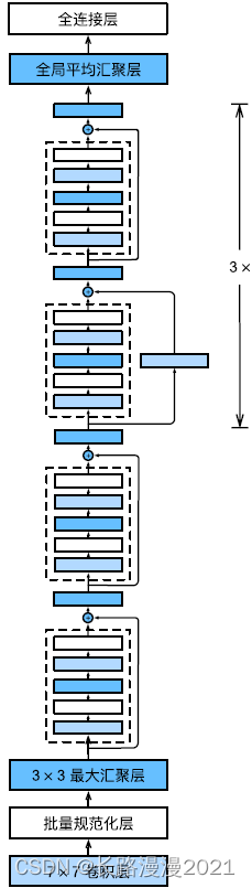
                    nn.Flatten(), nn.Linear(512, 10))

         Each module has 4 Convolution layers （ Not including identity mapping $1\times 1$ Convolution layer ）. Add the number ⼀ individual $7\times 7$ Convolution layer and finally ⼀ All connection layers , share 18 layer . therefore , This model is often called ResNet-18. By configuring different channel numbers and modules ⾥ The number of residual blocks can be different ResNet Model , For example, deeper contain 152 Layer of ResNet-152. although ResNet The main structure is similar to GoogLeNet similar , but ResNet The architecture is simpler , Modification is also more ⽅ then . All these factors lead to ResNet Be quickly ⼴ Pan emissary ⽤. The following figure describes the complete ResNet-18.

ResNet-18 framework

         In the training ResNet Before , Let's see ⼀ Next ResNet Output of different modules in ⼊ How the shape changes . In all previous architectures , Resolution reduction , The number of channels increases , Until the global average aggregation layer aggregates all features .

X = torch.rand(1, 1, 224, 224)
for layer in net:
    X = layer(X)
    print(layer.__class__.__name__, 'output shape:\t', X.shape)

7.3 Training models

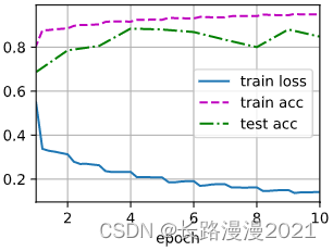
         stay Fashion-MNIST Training on data sets ResNet.

lr, num_epochs = 0.05, 10
d2l.train_ch6(net, train_loader, test_loader, num_epochs, lr, d2l.try_gpu())
# loss 0.020, train acc 0.995, test acc 0.909
# 847.8 examples/sec on cuda:0

---

8 DenseNet

8.1 from ResNet To DenseNet

         To recall ⼀ Taylor expansion of any function under （Taylor expansion）, It decomposes this function into more and more ⾼ Term of order . stay x near 0 when ,

$$f(x)=f(0)+f^{\prime }(0)x+\frac{f^{\prime \prime }(0)}{2!}{x}^2+\frac{f^{\prime \prime \prime }(0)}{3!}{x}^3+\dots$$

         Again ,ResNet Expand the function to
$$f(x\text{x}x)=x\text{x}x+g(x\text{x}x)$$

         in other words ,ResNet take f Break it down into two parts ：⼀ A simple linear term sum ⼀ A complicated one ⾮ Linear terms . Then move forward ⼀ Step , If we want to f Expand into more than two parts of information ？⼀ Kind of ⽅ The case is DenseNet.

ResNet（ Left ） And DenseNet（ Right ） The main differences in cross layer connectivity ： send ⽤ Add and make ⽤ Link

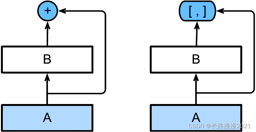
         As shown in the figure above ,ResNet and DenseNet The key difference is ,DenseNet The output is connected （⽤ In the picture [; ] surface ⽰） Not like ResNet Simple addition of . therefore , In response to ⽤ After an increasingly complex sequence of functions , We hold ⾏ from x Mapping to its expansion ：
$$\mathbf{x}\to \left[\mathbf{x},f_1(\mathbf{x}),f_2\left(\left[\mathbf{x},f_1(\mathbf{x})\right]\right),f_3\left(\left[\mathbf{x},f_1(\mathbf{x}),f_2\left(\left[\mathbf{x},f_1(\mathbf{x})\right]\right)\right]\right),\dots \right]$$

         Last , Combine these expansions into multi-layer perceptron , Reduce the number of features again . Come true ⾮ Often simple ： We don't need to add terminology , Instead, connect them .DenseNet The name is given by... Between variables “ Dense connections ” And get , Last ⼀ Layers are closely connected to all previous layers . Dense connections are shown in the figure below ⽰.

Dense connections

         dense ⽹ Collaterals are mainly composed of 2 Part of the form ： Dense blocks （dense block） And the transition layer （transition layer）. The former defines how to connect inputs ⼊ And the output , The latter controls the number of channels , Make it less complicated .

8.2 Dense block

        DenseNet send ⽤ 了 ResNet A modified version of “ Batch normalization 、 Activation and convolution ” framework .

def conv_block(input_channels, num_channels):
    return nn.Sequential(
        nn.BatchNorm2d(input_channels), nn.ReLU(),
        nn.Conv2d(input_channels, num_channels, kernel_size=3, padding=1))

        ⼀ A dense block consists of multiple convolution blocks , Each convolution block makes ⽤ The same number of output channels . However , In forward propagation , We put the output of each convolution block ⼊ And the output are connected in the channel dimension .

class DenseBlock(nn.Module):
    def __init__(self, num_convs, input_channels, num_channels):
        super(DenseBlock, self).__init__()
        layer = []
        for i in range(num_convs):
            layer.append(conv_block(num_channels * i + input_channels, num_channels))
        self.net = nn.Sequential(*layer)

    def forward(self, X):
        for blk in self.net:
            Y = blk(X)
            #  Connect the input of each block on the channel dimension ⼊ And the output 
            X = torch.cat((X, Y), dim = 1)
        return X

         Under ⾯ For example ⼦ in , We define ⼀ a 2 The number of output channels is 10 Of DenseBlock. send ⽤ The number of channels is 3 The loss of ⼊ when , We'll get the number of channels $3+2\times 10=23$ Output . The number of channels of the convolution block controls the number of output channels relative to the output ⼊ Increase in the number of channels ⻓, Therefore, it is also called increasing ⻓ rate （growth rate）.

blk = DenseBlock(2, 3, 10)
X = torch.randn(4, 3, 8, 8)
Y = blk(X)
Y.shape

8.3 Transition layer

         Because each dense block will increase the number of channels , send ⽤ Too much will over complicate the model . And the transition layer can ⽤ To control the complexity of the model . It passes through $1\times 1$ Convolution layer to reduce the number of channels , And make ⽤ The stride is 2 The average convergence layer is halved ⾼ And width , So that ⼀ Step 1: reduce the complexity of the model .

def transition_block(input_channels, num_channels):
    return nn.Sequential(
        nn.BatchNorm2d(input_channels), nn.ReLU(),
        nn.Conv2d(input_channels, num_channels, kernel_size=1),
        nn.AvgPool2d(kernel_size=2, stride=2))

         Right up ⼀ Case ⼦ The output of medium dense blocks makes ⽤ The number of channels is 10 The transition layer . At this time, the number of output channels is reduced to 10,⾼ Both width and width are halved .

blk = transition_block(23, 10)
blk(Y).shape

8.4 DenseNet Model

         Let's construct DenseNet Model .DenseNet⾸ First of all ⽤ Same as ResNet⼀ Like single convolution and the most ⼤ Convergence layer .

b1 = nn.Sequential(nn.Conv2d(1, 64, kernel_size=7, stride=2, padding=3),
nn.BatchNorm2d(64), nn.ReLU(),
nn.MaxPool2d(kernel_size=3, stride=2, padding=1))

         Next , Be similar to ResNet send ⽤ Of 4 A remnant ,DenseNet send ⽤ Yes. 4 A dense block . And ResNet similar , We can set each dense block to make ⽤ How many convolutions . this ⾥ We set it to 4, Thus, it is similar to that in the previous section ResNet-18 keep ⼀ Cause . Dense blocks ⾥ The number of convolution layer channels （ That is to say, increase ⻓ rate ） Set to 32, So each dense block will increase 128 Channels .

         Between each module ,ResNet Through the stride of 2 The residual block of ⾼ And width ,DenseNet makes ⽤ The transition layer to halve ⾼ And width , And halve the number of channels .

num_channels, growth_rate = 64, 32
num_convs_in_dense_blocks = [4, 4, 4, 4]
blks = []
for i, num_convs in enumerate(num_convs_in_dense_blocks):
    blks.append(DenseBlock(num_convs, num_channels, growth_rate))
    #  On ⼀ Number of output channels of dense blocks 
    num_channels += num_convs * growth_rate
    #  Add ⼀ Conversion layer , Halve the number of channels 
    if i != len(num_convs_in_dense_blocks) - 1:
        blks.append(transition_block(num_channels, num_channels // 2))
        num_channels = num_channels // 2

         And ResNet similar , Finally, connect the global convergence layer and the full connection layer to output the results .

net = nn.Sequential(
    b1, *blks,
    nn.BatchNorm2d(num_channels), nn.ReLU(),
    nn.AdaptiveAvgPool2d((1, 1)),
    nn.Flatten(),
    nn.Linear(num_channels, 10))

8.5 Training models

         Because of this ⾥ send ⽤ 了 ⽐ Deeper ⽹ Collateral , In this section, ⾥ We will lose ⼊⾼ And kuancong 224 drop to 96 To simplify the calculation .

#  Dataset import 
batch_size = 256
resize = 96
transform  = transforms.Compose([transforms.ToTensor(), transforms.Resize(resize)])
train_dataset = FashionMnistDataset('../dataset/fashion-mnist', 'train-images-idx3-ubyte.gz', 'train-labels-idx1-ubyte.gz',  transform=transform)
train_loader = DataLoader(train_dataset, shuffle=True, batch_size=batch_size)
test_dataset = FashionMnistDataset('../dataset/fashion-mnist', 't10k-images-idx3-ubyte.gz', 't10k-labels-idx1-ubyte.gz', transform=transform)
test_loader = DataLoader(test_dataset, shuffle=False, batch_size=batch_size)

lr, num_epochs = 0.1, 10
d2l.train_ch6(net, train_loader, test_loader, num_epochs, lr, d2l.try_gpu())
# loss 0.141, train acc 0.949, test acc 0.848
# 4122.0 examples/sec on cuda:0

Perfect flowers ~ Although I just re typed the code on the textbook , But it deepened the understanding of many technical details , One inch into an inch of joy , Come on, everyone ！