当前位置:网站首页>[beauty of algebra] solution method of linear equations ax=0
[beauty of algebra] solution method of linear equations ax=0
2022-07-05 08:55:00 【Li Yingsong~】
stay 3D In vision , We often encounter such a problem : Solve linear equations A x = 0 Ax=0 Ax=0, From the perspective of matrix mapping , All solutions form a matrix A A A Zero space of . A typical scenario, such as using the eight point method to solve the essential matrix E E E, See my previous blog : Introduction to stereo vision (2): Key matrix ( The essential matrix , Basic matrix , Homography matrix ). This is a basic and common linear algebra problem , In this article, we will discuss the solution of this kind of problem , It is also an introductory course .
List of articles
The obvious solution
about A x = 0 Ax=0 Ax=0, Obviously , x = 0 x=0 x=0 It must be one of the solutions , But for our practical application , Getting a zero solution is often meaningless , So no discussion .
Nonzero special solution
As mentioned earlier , What we actually want , Nonzero solution , They are obviously deeper than the zero solution .
Before discussing nonzero solutions , We must introduce the concept of special solution . One obvious point is , A x = 0 Ax=0 Ax=0 The scale is constant , I.e x s x_s xs Is one of the solutions , be k s x s k_sx_s ksxs It must also be the solution ( k s k_s ks Is the set of real Numbers ), and k s x s k_sx_s ksxs and x s x_s xs It's linear ; Further , If x t x_t xt It's another one with x s x_s xs Linearly independent solutions , namely
A x s = 0 , A x t = 0 , x s and x t Line sex nothing Turn off Ax_s=0,Ax_t=0,x_s and x_t Linearly independent Axs=0,Axt=0,xs and xt Line sex nothing Turn off
Obviously A ( k s x s + k t x t ) = 0 A(k_sx_s+k_tx_t)=0 A(ksxs+ktxt)=0 It's also true ( k s , k t k_s,k_t ks,kt Is the set of real Numbers ), namely k s x s + k t x t k_sx_s+k_tx_t ksxs+ktxt It's also the solution of the equation . This reveals a phenomenon : If the equations A x = 0 Ax=0 Ax=0 There are several linearly independent solutions x 1 , x 2 , . . . , x n x_1,x_2,...,x_n x1,x2,...,xn, be x 1 , x 2 , . . . , x n x_1,x_2,...,x_n x1,x2,...,xn Any linear combination of is also its solution , let me put it another way , All solutions can pass x 1 , x 2 , . . . , x n x_1,x_2,...,x_n x1,x2,...,xn Linear combination . Let's take these linear independent solutions x 1 , x 2 , . . . , x n x_1,x_2,...,x_n x1,x2,...,xn It is called a system of equations A x = 0 Ax=0 Ax=0 Special solution of .
therefore , Our purpose , In fact, we need to calculate all non-zero special solutions .
First of all, we want to find out , How many non-zero special solutions are there ?
We analyze it from the elimination and substitution solution , Suppose a matrix A ∈ R m × n ( m = 3 , n = 4 ) A\in R^{m\times n}(m=3,n=4) A∈Rm×n(m=3,n=4):
A = [ 1 3 6 6 2 2 4 8 4 4 8 16 ] A=\left[\begin{matrix}1&3&6&6\\2&2&4&8\\4&4&8&16\end{matrix}\right] A=⎣⎡1243246486816⎦⎤
First of all, A A A Carry out elimination ,
[ 1 3 6 6 2 2 4 8 4 4 8 16 ] → [ 1 3 6 6 2 2 4 8 0 0 0 0 ] → [ 1 3 6 6 0 2 4 2 0 0 0 0 ] \left[\begin{matrix}1&3&6&6\\2&2&4&8\\4&4&8&16\end{matrix}\right]\rightarrow\left[\begin{matrix}1&3&6&6\\2&2&4&8\\0&0&0&0\end{matrix}\right]\rightarrow\left[\begin{matrix}\boxed1&3&6&6\\0&\boxed2&4&2\\0&0&0&0\end{matrix}\right] ⎣⎡1243246486816⎦⎤→⎣⎡120320640680⎦⎤→⎣⎡100320640620⎦⎤
In the matrix after elimination , In box 1 and 2 It is called the primary variable (pivot variable), Also known as principal . The number of principal elements is called the rank of the matrix , The number of principal elements here is 2, So the matrix A The rank of (rank) Also for the 2, namely r a n k ( A ) = 2 rank(A)=2 rank(A)=2.
The column in which the primary element is located is called the primary column (pivot column), The main columns here are 1 Column and the first 2 Column , Other columns 3 Column and the first 4 List as free column (free column). The variables in the free column are free variables (free variable), The number of free variables is n − r a n k ( A ) = 4 − 2 = 2 n-rank(A)=4-2=2 n−rank(A)=4−2=2.
According to the elimination solution , After elimination, we assign values to free variables , Back substitution to find the value of the main column variable . Give free variables respectively [ x 3 x 4 ] \left[\begin{matrix}x_3\\x_4\end{matrix}\right] [x3x4] The assignment is [ 1 0 ] \left[\begin{matrix}1\\0\end{matrix}\right] [10] and [ 0 1 ] \left[\begin{matrix}0\\1\end{matrix}\right] [01], The following two solution vectors are obtained by substituting the equation :
[ 0 − 2 1 0 ] , [ − 3 − 1 0 1 ] \left[\begin{matrix}0\\-2\\1\\0\end{matrix}\right],\left[\begin{matrix}-3\\-1\\0\\1\end{matrix}\right] ⎣⎢⎢⎡0−210⎦⎥⎥⎤,⎣⎢⎢⎡−3−101⎦⎥⎥⎤
These two solution vectors are linear equations A x = 0 Ax=0 Ax=0 Two non-zero special solutions of , Other solutions can be expressed linearly by these two solutions : x = a [ 0 − 2 1 0 ] + b [ − 3 − 1 0 1 ] x=a\left[\begin{matrix}0\\-2\\1\\0\end{matrix}\right]+b\left[\begin{matrix}-3\\-1\\0\\1\end{matrix}\right] x=a⎣⎢⎢⎡0−210⎦⎥⎥⎤+b⎣⎢⎢⎡−3−101⎦⎥⎥⎤. It can also be said that any linear combination of special solutions constructs a matrix A A A The whole zero space of .
You know , System of linear equations A x = 0 Ax=0 Ax=0 The number of non-zero special solutions of is n − r a n k ( A ) n-rank(A) n−rank(A).
Least square solution
The above analysis is only from the perspective of Pure Mathematics , But in the application of Computer Science , The most common situation we encounter is , Through a large number of observations with certain noise , The number of construction equations is much larger than the unknown Overdetermined linear equations A x = 0 , A ∈ R m × n , m ≫ n Ax=0,A\in R^{m\times n},m\gg n Ax=0,A∈Rm×n,m≫n, At this time, there is often no strict solution .
For example, in solving the essential matrix of two images E E E when , We will match a large number of feature point pairs , Then linear equations are constructed based on antipolar constraints A e = 0 Ae=0 Ae=0 Solve the element vector of the essential matrix e e e, The number of characteristic point pairs is often far more than the number of elements of the essential matrix ( namely m ≫ n m\gg n m≫n), And because of the existence of point noise , The antipolar constraint is not strictly established ( namely A x ≈ 0 Ax\approx 0 Ax≈0). In the face of this situation , Our usual practice is to ask Least square solution . namely :
x ^ = arg min x ∣ ∣ A x ∣ ∣ 2 2 \hat {x}=\arg\min_x||Ax||_2^2 x^=argxmin∣∣Ax∣∣22
But we immediately found a problem , Scale invariance as mentioned above , If x s x_s xs It's a solution , be k s x s k_sx_s ksxs It's also the solution , Then when we find a solution , Infinitely reduce the module length of the solution vector , ∣ ∣ A x ∣ ∣ 2 2 ||Ax||_2^2 ∣∣Ax∣∣22 Wouldn't it be infinitely small , Which one should I choose ? This is obviously an impasse .
therefore , We're going to give x x x A constraint , That is, its module length is limited to a constant , For example, the most commonly used unit module length 1, namely x x x Must satisfy , ∣ ∣ x ∣ ∣ 2 2 = 1 ||x||_2^2=1 ∣∣x∣∣22=1. This reconstructs a constrained least squares problem :
x ^ = arg min x ∣ ∣ A x ∣ ∣ 2 2 , subject to ∣ ∣ x ∣ ∣ 2 2 = 1 \hat {x}=\arg\min_x||Ax||_2^2,\text{subject to} ||x||_2^2=1 x^=argxmin∣∣Ax∣∣22,subject to∣∣x∣∣22=1
According to the Lagrange multiplier method , another
L ( x , λ ) = ∣ ∣ A x ∣ ∣ 2 2 + λ ( 1 − ∣ ∣ x ∣ ∣ 2 2 ) L(x,\lambda)=||Ax||_2^2+\lambda(1-||x||_2^2) L(x,λ)=∣∣Ax∣∣22+λ(1−∣∣x∣∣22)
requirement L ( x , λ ) L(x,\lambda) L(x,λ) minimum value , Then first find the extreme value , That is, the first partial derivative is 0 The point of , We are respectively right x , λ x,\lambda x,λ Find the partial derivative and make it equal to 0:
L ′ ( x ) = 2 A T A x − 2 λ x = 0 L ′ ( λ ) = 1 − x T x = 0 \begin{aligned} L^{'}(x)&=2A^TAx-2\lambda x=0\\ L^{'}(\lambda)&=1-x^Tx=0 \end{aligned} L′(x)L′(λ)=2ATAx−2λx=0=1−xTx=0
Then there are A T A x = λ x A^TAx=\lambda x ATAx=λx, This familiar formula tells us , x x x It's a matrix A T A A^TA ATA The characteristic value is λ \lambda λ Eigenvector of .
But the matrix A T A A^TA ATA At most n n n Eigenvalues , Corresponding n n n eigenvectors , Which is the minimum point ?
Let's make another derivation : When x x x It's a matrix A T A A^TA ATA The characteristic value is λ \lambda λ When the eigenvector of , Yes
∣ ∣ A x ∣ ∣ 2 2 = x T A T A x = x T λ x = λ x T x = λ ||Ax||_2^2=x^TA^TAx=x^T\lambda x=\lambda x^Tx=\lambda ∣∣Ax∣∣22=xTATAx=xTλx=λxTx=λ
therefore , When λ \lambda λ Take the minimum , ∣ ∣ A x ∣ ∣ 2 2 ||Ax||_2^2 ∣∣Ax∣∣22 Minimum value , namely Least square solution x ^ \hat{x} x^ It's a matrix A T A A^TA ATA The eigenvector corresponding to the minimum eigenvalue . This is a system of overdetermined linear equations A x = 0 Ax=0 Ax=0 The least square solution of .
边栏推荐
- Digital analog 1: linear programming
- How to manage the performance of R & D team?
- 微信H5公众号获取openid爬坑记
- Latex improve
- 深度学习模型与湿实验的结合,有望用于代谢通量分析
- [matlab] matlab reads and writes Excel
- Halcon color recognition_ fuses. hdev:classify fuses by color
- JS asynchronous error handling
- Halcon shape_ trans
- TF coordinate transformation of common components of ros-9 ROS
猜你喜欢

RT-Thread内核快速入门,内核实现与应用开发学习随笔记

Beautiful soup parsing and extracting data
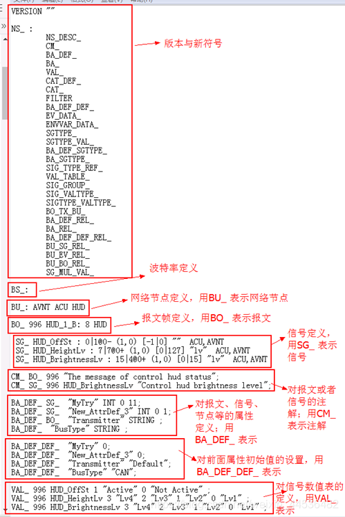
AUTOSAR从入门到精通100讲(103)-dbc文件的格式以及创建详解
2020 "Lenovo Cup" National College programming online Invitational Competition and the third Shanghai University of technology programming competition
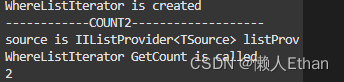
Count of C # LINQ source code analysis
容易混淆的基本概念 成员变量 局部变量 全局变量
The combination of deep learning model and wet experiment is expected to be used for metabolic flux analysis
Introduction Guide to stereo vision (1): coordinate system and camera parameters
C# LINQ源码分析之Count
Digital analog 1: linear programming
随机推荐
深度学习模型与湿实验的结合,有望用于代谢通量分析
How to manage the performance of R & D team?
Halcon shape_ trans
asp. Net (c)
Halcon: check of blob analysis_ Blister capsule detection
Multiple linear regression (gradient descent method)
TF coordinate transformation of common components of ros-9 ROS
How many checks does kubedm series-01-preflight have
Return of missing persons
The first week of summer vacation
牛顿迭代法(解非线性方程)
多元线性回归(梯度下降法)
JS asynchronous error handling
多元线性回归(sklearn法)
Summary of "reversal" problem in challenge Programming Competition
RT thread kernel quick start, kernel implementation and application development learning with notes
12. Dynamic link library, DLL
Ros-11 common visualization tools
Causes and appropriate analysis of possible errors in seq2seq code of "hands on learning in depth"
【日常訓練--騰訊精選50】557. 反轉字符串中的單詞 III