当前位置:网站首页>[LZY learning notes -dive into deep learning] math preparation 2.5-2.7
[LZY learning notes -dive into deep learning] math preparation 2.5-2.7
2022-07-03 10:18:00 【DadongDer】
2.5 Automatic differentiation
Deep learning framework through ⾃ Calculate the derivative dynamically , namely ⾃ Dynamic differential (automatic differentiation) To speed up the derivation . In the actual , According to the model we designed , The system will build ⼀ Calculation charts (computational graph), To track which data is calculated and which operations are combined to produce ⽣ Output .
⾃ Dynamic differentiation enables the system to subsequently Back propagation gradient . this ⾥, Back propagation (backpropagate) It means tracking the whole calculation diagram , Fill in the partial derivative of each parameter .
Sharing by a netizen , Explain the calculation diagram and BP
An example
import torch

x = torch.arange(4.0)

#  Not every time ⼀ Allocate new memory when deriving parameters
#  Because we often update the same parameters thousands of times , Allocating new memory every time may soon run out of memory
#  A scalar function about a vector x The gradient of is with x Vectors of the same shape
x.requires_grad_(True)
#  Equivalent to  x=torch.arange(4.0,requires_grad=True)
print(x.grad)

y = 2 * torch.dot(x,x) # y = 2 x⊤ x
print(y)

#  Call the back propagation function to automatically calculate y About x The gradient of each component
y.backward()
print(x.grad)

# f(x) = 2*x0*x0 + 2*x1*x1 + 2*x2*x2 + 2*x3*x3
# df(x)/dx0 = 4*x0 when x0 = 0, df(x)/dx0 = 0
# df(x)/dx1 = 4*x1 when x1 = 1, df(x)/dx0 = 4
# df(x)/dx2 = 4*x2 when x2 = 2, df(x)/dx0 = 8
# df(x)/dx3 = 4*x3 when x3 = 4, df(x)/dx0 = 12

print(x.grad == 4*x)

#  By default ,PyTorch It accumulates gradients , We need to clear the previous value
x.grad.zero_()
y = x.sum()
# f(x) = x0 + x1 + x2 + x3
# df(x)/dx0 = df(x)/dx1 = df(x)/dx2 = df(x)/dx3 = 1
y.backward()
print(x.grad)
Back propagation of non scalar variables
When y When it's not scalar , vector y About vectors x The derivative of ⾃ However, the explanation is ⼀ Matrix . about ⾼ Step sum ⾼ Dimensional y and x, The result of derivation can be ⼀ individual ⾼ Order tensor .
Gradient in partial derivative of Advanced Mathematics , The gradient indicates the direction in which a scalar function rises or falls most violently at a certain point and the directional derivative of that direction .
x = torch.arange(4.0,requires_grad=True)
y = x * x #  By element
#  Yes ⾮ Scalar modulation ⽤backward Need to transmit ⼊⼀ individual gradient Parameters , This parameter specifies the differential function about self Gradient of .
#  Just want to find the sum of partial derivatives , So deliver ⼀ individual 1 The gradient of is appropriate  ( ride 1 Adding up is sum)
y.sum().backward()      # y.backward(torch.ones(len(x)))
print(x.grad)
Separation of computing
You want to move some calculations out of the recorded calculation graph .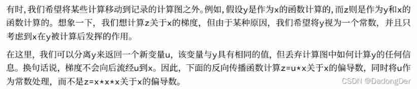
import torch

x = torch.arange(4.0,requires_grad=True)
y = x * x #  Non scalar
u = y.detach()
z = u * x #  Non scalar
z.sum().backward()
print(x.grad == u) # tensor([True, True, True, True])

x.grad.zero_()
y.sum().backward() #  Non scalar
print(x.grad == 2 * x) # tensor([True, True, True, True])
Python Gradient calculation of control flow
send ⽤⾃ Dynamic differential ⼀ One advantage is that : Even if the calculation diagram of the construction function needs to pass Python control flow ( for example , Conditions 、 Loop or any function call ), We can still calculate the gradient of the variable .
import torch
def f(a):
    b = a * 2
    while b.norm() < 1000:
        b = b * 2
    if b.sum() > 0:
        c = b
    else:
        c = 100 * b
    return c

a = torch.randn(size=(), requires_grad=True)
d = f(a)
d.backward()
print(a.grad == d / a)
# tensor(True)
Summary
Deep learning framework can ⾃ Calculate the derivative dynamically : We first attach the gradient to the variable on which we want to calculate the partial derivative . Then we record ⽬ Calculation of benchmark value , Execute its back propagation function , And access the resulting gradient .
2.6 probability
Basic probability theory
The process of sampling from the probability distribution is called sampling (sampling)
Assign probability to ⼀ The distribution of some discrete choices is called multinomial distribution (multinomial distribution)
In estimation ⼀ Dice ⼦ The fairness of , We hope from the same ⼀ In distribution ⽣ Into multiple samples . If ⽤Python Of for Loop to complete the task , The speed will be surprisingly slow ⼈. So we make ⽤ The function of the deep learning framework extracts multiple samples at the same time , Get any shape we want ⽴ Sample array .
import torch
from torch.distributions import multinomial
import matplotlib.pyplot as plt
# A probability distribution
fair_probs = torch.ones([6]) / 6
# Sample the data / Sampling
# sample 600 times with fair probs. theoritical output [100, 100, 100, 100, 100, 100]
print(multinomial.Multinomial(600, fair_probs).sample())
# Calculate the relative frequency as an estimate of the true probability
counts = multinomial.Multinomial(1000, fair_probs).sample()
print(counts / 1000) # theoritical value: 1/6 ~= 0.167
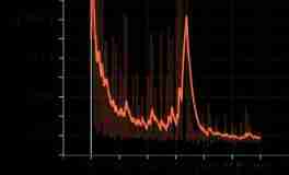
# How the probability converges to the real probability over time
# Into the ⾏500 Group experiment , Extraction of each group 10 Samples
counts = multinomial.Multinomial(10, fair_probs).sample((500,))
cum_counts = counts.cumsum(dim=0) # Add by line
estimates = cum_counts / cum_counts.sum(dim=1, keepdims=True) # Keep the shape without dimension reduction
print(estimates)
# draw 6 line
for i in range(6):
plt.plot(estimates[:, i].numpy(), label=("P(die=" + str(i + 1) + ")"))
plt.axhline(y=0.167, color='black', linestyle='dashed') # axhline Draw parallel to x Horizontal reference line of axis
plt.gca().set_xlabel("Groups of experiments")
plt.gca().set_ylabel("Estimated probability")
plt.legend() # Add icons
plt.show()
axiom :
When processing the roll of dice , We will gather S = {1, 2, 3, 4, 5, 6} Called sample space (sample space) Or result space (outcome
space), Each of these elements is the result (outcome)
event (event) yes ⼀ Random results of a given set of sample spaces 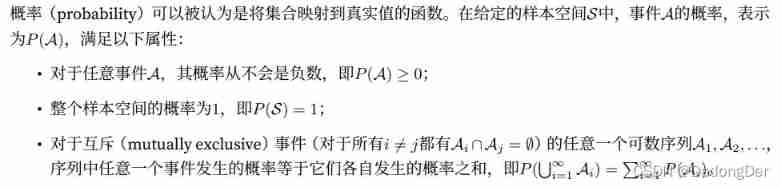
A random variable :
Discrete random variable vs Continuous random variables ( Section )
In these cases , We quantify the probability of seeing a certain value as density (density). The height is just 1.80 The probability of meters is 0, But density is not 0.
Handle multiple random variables
① joint probability joint probability P(A = a, B = b)
A = a and B = b At the same time ⽣ The possibility is not ⼤ On A = a or B = b Single issue ⽣ The possibility of
② Conditional probability conditional probability
③ Bayes theorem Bayes’theorem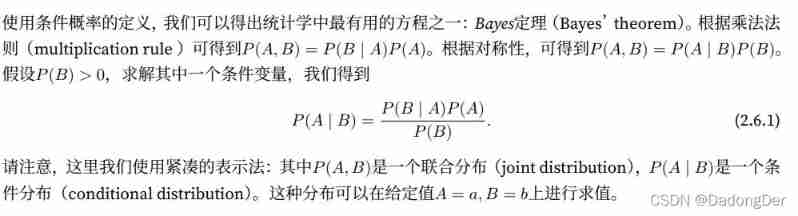
④ Marginalization 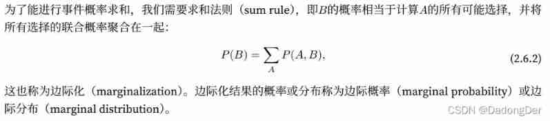
⑤ independence
rely on (dependence) And alone ⽴(independence)
If two random variables A and B It's the only one ⽴ Of , It means events A The hair of ⽣ Follow B The occurrence of events ⽣⽆ Turn off .
Two random variables are unique ⽴ Of , If and only if the joint distribution of two random variables is their respective ⾃ The product of the distribution .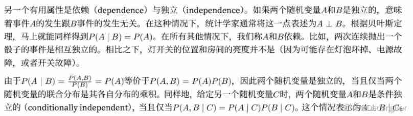
Expectation and variance : Summarize the key characteristics of probability distribution 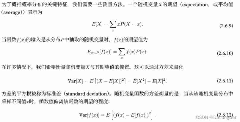
⼩ junction
• We can sample from the probability distribution .
• We can make ⽤ Joint distribution 、 Conditional distribution 、Bayes Theorem 、 Marginalization and independence ⽴ Sex hypothesis to analyze multiple random variables .
• Expectations and ⽅ Difference provides a real basis for the generalization of the key characteristics of probability distribution ⽤ Measurement form of .
2.7 Consult the documentation
Find all functions and classes in the module
Usually , We can ignore it by “__”( Double underline ) Start and end functions ( They are Python Special objects in ), Or in a single “_”( Underline ) Start function ( They are usually internal functions ).
import torch
#  see PyTorch API Guidance of

#  Query random numbers ⽣ All attributes in the module
print(dir(torch.distributions)) #  Adjustable in the module ⽤ Which functions and classes
Find the usage of specific functions and classes
import torch
#  How to make ⽤ A more specific description of a given function or class

#  Look at the tensor ones function
help(torch.ones)
⼩ junction
• Officer, ⽅⽂ Files provide information beyond this book ⼤ Quantity description and ⽰ example .
• We can adjust ⽤dir and help Function or in Jupyter Make... In Notepad ⽤? and ?? see API Of ⽤ Law ⽂ files .
边栏推荐
- getopt_ Typical use of long function
- 1. Finite Markov Decision Process
- 20220609其他:多数元素
- After clicking the Save button, you can only click it once
- 2.2 DP: Value Iteration & Gambler‘s Problem
- Leetcode - 5 longest palindrome substring
- LeetCode - 460 LFU 缓存(设计 - 哈希表+双向链表 哈希表+平衡二叉树(TreeSet))*
- CV learning notes - scale invariant feature transformation (SIFT)
- CV learning notes - clustering
- 『快速入门electron』之实现窗口拖拽
猜你喜欢

Discrete-event system
Deep Reinforcement learning with PyTorch

Opencv note 21 frequency domain filtering
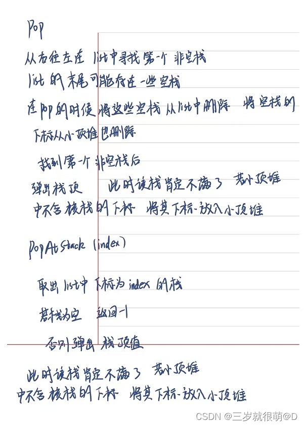
LeetCode - 1172 餐盘栈 (设计 - List + 小顶堆 + 栈))
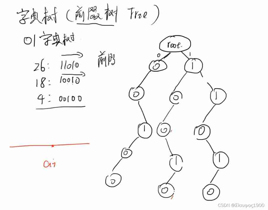
Dictionary tree prefix tree trie

Opencv histogram equalization

CV learning notes - edge extraction

Mise en œuvre d'OpenCV + dlib pour changer le visage de Mona Lisa

Swing transformer details-2

Connect Alibaba cloud servers in the form of key pairs
随机推荐
Basic use and actual combat sharing of crash tool
The data read by pandas is saved to the MySQL database
4G module initialization of charge point design
CV learning notes - Stereo Vision (point cloud model, spin image, 3D reconstruction)
一步教你溯源【钓鱼邮件】的IP地址
Label Semantic Aware Pre-training for Few-shot Text Classification
20220608 other: evaluation of inverse Polish expression
openCV+dlib實現給蒙娜麗莎換臉
Policy Gradient Methods of Deep Reinforcement Learning (Part Two)
LeetCode - 460 LFU 缓存(设计 - 哈希表+双向链表 哈希表+平衡二叉树(TreeSet))*
2312、卖木头块 | 面试官与狂徒张三的那些事(leetcode,附思维导图 + 全部解法)
20220607 others: sum of two integers
What did I read in order to understand the to do list
Simulate mouse click
Leetcode - 1670 conception de la file d'attente avant, moyenne et arrière (conception - deux files d'attente à double extrémité)
My notes on the development of intelligent charging pile (III): overview of the overall design of the system software
Leetcode 300 最长上升子序列
20220605 Mathematics: divide two numbers
LeetCode - 900. RLE iterator
CV learning notes - edge extraction