当前位置:网站首页>Common machine learning related evaluation indicators
Common machine learning related evaluation indicators
2022-07-02 07:36:00 【wxplol】
Catalog
Two 、 Confusion matrix Confusion Matrix
3、 ... and 、Precision( accuracy ) and Recall( Recall rate )
5、 ... and 、PR curve 、ROC curve
7、 ... and 、 Return to (Regression) Algorithm index
8、 ... and 、 Deep learning target detection related indicators
8.1、IOU Occurring simultaneously than
8.2、NMS Non maximum suppression
In the process of using machine learning model , We inevitably encounter how to evaluate whether our model is good or bad ? Or when we read other people's papers , There will always be some, such as :“ Accuracy rate ”、“ Recall rate ” Things like that . Bloggers have a bad memory and always forget to distinguish foolishly , Always confused . therefore , Record some common evaluation indicators here , The following figure shows the evaluation indicators of different machine learning algorithms :

One 、Accuracy Accuracy rate
Divide the number of samples in the detection time by the number of all samples . Accuracy is generally used to evaluate the global accuracy of the detection model , Limited information contained , Cannot fully evaluate the performance of a model .
Two 、 Confusion matrix Confusion Matrix
For a binary task , The prediction results of two classifiers can be divided into the following 4 class :
- TP: true positive— Predict positive samples as positive
- TN:true negative— Predict negative samples as negative
- FP:false positive— Predict negative samples as positive
- FN:false negative— Predict positive samples as negative
Positive sample | Negative sample | |
| Positive sample ( forecast ) | TP( True positive ) | FP( False positive ) |
| Negative sample ( forecast ) | FN( false negative ) | TN( True negative ) |
3、 ... and 、Precision( accuracy ) and Recall( Recall rate )
For a sample of seriously unbalanced data , such as : mail , If we had 1000 Messages , Among them, normal mail 999 individual , And spam only 1 individual , Then assume that all samples are identified as normal emails , So at this time Accuracy by 99.9%. It looks like our model is good , But this model can't recognize spam , Because the purpose of training this model is to classify spam , Obviously, this is not the evaluation index of a model we need . Of course , In the actual model , We will use this indicator to preliminarily judge whether our model is good or bad .
Through the instructions above , We know that accuracy alone cannot accurately measure our model , So here we introduce Precision( accuracy ) and Recall( Recall rate ), they It is only applicable to two classification problems . Let's first look at its definition :
Precision( accuracy )
- Definition : The proportion of the number of positive examples correctly classified to the number of instances classified as positive examples , Also known as Precision rate .
- Calculation formula :


Recall( Recall rate )
- Definition : The proportion of the number of positive cases correctly classified to the actual number of positive cases Also known as Recall rate .
- Calculation formula :


Ideally , The higher the accuracy rate and recall rate, the better . However, in fact, the two are contradictory in some cases , When the accuracy is high , Low recall rate ; When the accuracy is low , High recall rate ; About this property through observation PR The curve is not difficult to observe . For example, when searching the web , If only the most relevant web page is returned , The accuracy is 100%, And the recall rate is very low ; If you go back to the full page , What's the recall rate 100%, The accuracy is very low . Therefore, in different occasions, we need to judge which index is important according to the actual needs .
Four 、 Fβ Score
Usually , The precision rate and recall rate affect each other ,Precision high 、Recall Is low ;Recall high 、Precision Is low . Is there a way to measure these two indicators ? So here comes F1 Score.F1 Function is a common indicator ,F1 The value is the harmonic mean of accuracy and recall , namely


Of course ,F The value can be generalized to give different weights to the accuracy rate and recall rate for weighted reconciliation :

among ,β>1 when , Recall is more influential ;β=1 when , Degenerate into standard F1;β<1 when , The accuracy rate is more influential .
5、 ... and 、PR curve 、ROC curve
5.1、PR curve
PR Curve to Precision( accuracy ) Vertical coordinates ,Recall( Recall rate ) Abscissa . As shown in the figure below :

It's not hard to see from the above picture that ,precision And Recall A compromise of (trade off), The closer the curve is to the upper right corner, the better the performance , The area under the curve is called AP fraction , To a certain extent, it can reflect the high proportion of accuracy rate and recall rate of the model . But this value is not easy to calculate , Considering the accuracy and recall rate, it is generally used F1 Function or AUC value ( because ROC Curves are easy to draw ,ROC The area under the curve is also easier to calculate ).
Generally speaking , Use PR The curve evaluates the quality of a model , First look at the smoothness , Watching who goes up and who goes down ( On the same test set ), Generally speaking , The top one is better than the bottom one ( The red line is better than the black line ).
5.2、ROC curve
Among many machine learning models , Many models output prediction probability , And use accuracy 、 When evaluating the model with indicators such as recall , It is also necessary to set a classification threshold for the prediction probability , For example, if the prediction probability is greater than the threshold, it is a positive example , On the contrary, it is a negative example . This adds a super parameter to the model , And this super parameter will affect the generalization ability of the model .
ROC Curve curve does not need to set such a threshold ,ROC The ordinate of the curve is the true rate , The abscissa is the false positive rate , ROC(Receiver Operating Characteristic) Curves are often used to evaluate the merits of a binary classifier ,ROC The horizontal axis of is false positive rate,FPR,“ The false positive rate is ”, That is, the wrong proportion ; The vertical axis is true positive rate,TPR,“ True case rate ”, That is, the correct judgment is the correct proportion .
- Real class rate (True Postive Rate)TPR:
 , In all the positive samples , The classifier predicts the correct proportion ( be equal to Recall).
 - True negative class rate (True Negative Rate)FPR:
 , In all negative samples , The proportion of classifier prediction errors .
 , In all the positive samples , The classifier predicts the correct proportion ( be equal to Recall).
 , In all negative samples , The proportion of classifier prediction errors .
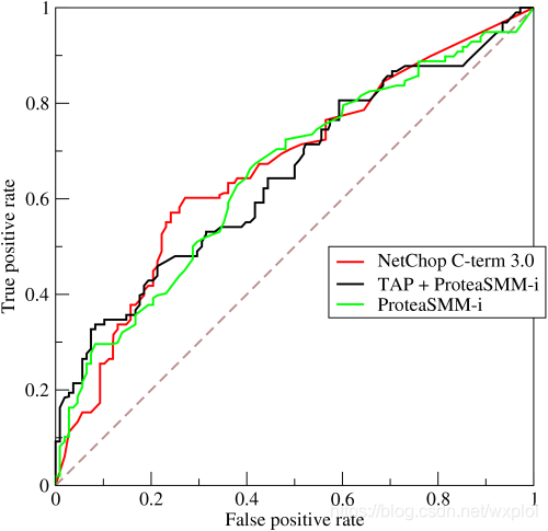
ROC The full name of a curve is Receiver Operating Characteristic, It is often used to judge the quality of a classifier .ROC The curve is FPR And TPR The relationship between , This combination FPR Yes TPR, At a price (costs) To income (benefits), Obviously, the higher the return , The lower the price , The better the performance of the model . The better the model works , Whole ROC The curve moves towards the upper left corner , And PR Similar to if a model ROC Complete curve cover the other one , It shows that this model is better than another model .
Another thing to note ,AUC The algorithm considers the classification ability of the learner for both positive and negative cases , In case of sample imbalance , Still able to make a reasonable evaluation of the classifier .AUC It is not sensitive to whether the sample categories are balanced , This is also an unbalanced sample, which is usually used AUC One reason to evaluate the performance of a learner .
AUC The fraction is the area under the curve (Area under curve), Larger means better classifier effect . Obviously, the value of this area will not be greater than 1. And because of ROC The curve is generally in y=x Above this straight line , therefore AUC The value range of is 0.5 and 1 Between . Use AUC Value as the evaluation standard is because many times ROC The curve doesn't clearly show which classifier works better , And as a number , Corresponding AUC Bigger classifiers work better .
Now that there are so many evaluation criteria , Why even use ROC and AUC Well ? because ROC The curve has a good property : When the distribution of positive and negative samples in the test set changes ,ROC The curve can stay the same . Class imbalance often occurs in the actual data set (class imbalance) The phenomenon , That is, the negative sample is much more than the positive sample ( Or vice versa ), And the distribution of positive and negative samples in the test data may also change over time .
6、 ... and 、AUC
AUC It's a model evaluation index , It can only be used for the evaluation of binary model , For binary models , There are many other evaluation indicators , such as logloss,accuracy,precision. If you often pay attention to data mining competitions , such as kaggle, Then you will find AUC and logloss Basic is the most common model evaluation index . Why? AUC and logloss Than accuracy More commonly used ? Because many machine learning models predict the classification problem with probability , If you want to calculate accuracy, You need to convert probability into categories first , This requires manually setting a threshold , If the prediction probability of a sample is higher than this prediction , Just put this sample into a category , Below this threshold , Put it in another category . So this threshold greatly affects accuracy The calculation of . Use AUC perhaps logloss It can avoid converting prediction probability into category .
AUC yes Area under curve An acronym for .AUC Namely ROC The area under the curve , A performance index to measure the quality of a learner . By definition ,AUC Can be based on ROC The area of each part under the curve is summed to obtain . Assume ROC The curve is made up of coordinates (x1,y1),...,(xm,ym) The points of are connected in order to form , be AUC It can be estimated as :

AUC The value is ROC The curve covers Area , obviously ,AUC The bigger it is , The better the classifiers are .
- AUC = 1, It's the perfect classifier .
- 0.5 < AUC < 1, Better than random guessing . It has predictive value .
- AUC = 0.5, It's like a random guess ( example : Lose the copper plate ), No predictive value .
- AUC < 0.5, Worse than a random guess ; But as long as it's always against prediction , Better than random guessing .
AUC The physical meaning of AUC The physical meaning of the positive sample is greater than the probability of the negative sample . therefore AUC The response is the ability of the classifier to sort the samples . Another thing to note ,AUC It is not sensitive to whether the sample categories are balanced , This is also an unbalanced sample, which is usually used AUC A reason for evaluating classifier performance .
How to calculate AUC?
- Law 1:AUC by ROC The area under the curve , Then we can calculate the area directly . The area is a small trapezoidal area ( curve ) The sum of the . The accuracy of the calculation is related to the accuracy of the threshold .
- Law 2: according to AUC The physical meaning of , We calculated The prediction result of positive samples is greater than that of negative samples Of probability . take n1* n0(n1 Is the positive number of samples ,n0 Is the number of negative samples ) Two tuples , Each binary compares the prediction results of positive samples and negative samples , If the prediction result of positive samples is higher than that of negative samples, the prediction is correct , The ratio of the correct binary to the total binary is the final result AUC. The time complexity is O(N* M).
- Law 3: Let's first take all the samples according to score Sort , In turn rank Show them , Like the biggest score The sample of ,rank=n (n=n0+n1, among n0 Is the number of negative samples ,n1 Is the number of positive samples ), Next is n-1. So for a positive sample rank The largest sample ,rank_max, Yes n1-1 Other positive samples score Small , Then there is (rank_max-1)-(n1-1) Negative sample ratio score Small . Next is (rank_second-1)-(n1-2). Finally, we get the probability that the positive sample is larger than the negative sample is :

among :
n0、n1—— The number of negative samples and positive samples
rank(score)—— On behalf of the i Serial number of the sample .( Probability score from small to large , In the first rank A place ). Here is to add up the serial numbers of all positive samples .
This paper focuses on the third calculation method , It is also recommended that you calculate AUC Choose this method . About how to calculate , Please refer to the following links , Just watch it once .
Reference link :AUC The calculation method of
Why do you say ROC and AUC Can be applied to unbalanced classification problems ?
ROC The curve is only related to the abscissa (FPR) and Ordinate (TPR) It matters . We can find out TPR Just the probability of correct prediction in positive samples , and FPR Just the probability of prediction error in negative samples , It has nothing to do with the proportion of positive and negative samples . therefore ROC The value of is independent of the actual positive and negative sample ratio , Therefore, it can be used for equilibrium problems , It can also be used for unbalanced problems . and AUC The geometric meaning of is ROC The area under the curve , Therefore, it has nothing to do with the actual proportion of positive and negative samples .
7、 ... and 、 Return to (Regression) Algorithm index
6.1、 Mean absolute error MAE
Mean absolute error MAE(Mean Absolute Error) Also known as L1 Norm loss .

MAE Although it can better measure the quality of the regression model , But the existence of absolute value makes the function not smooth , It's impossible to derive at some points , Consider changing the absolute value to the square of the residual , This is the mean square error .
6.2、 Mean square error MSE
Mean square error MSE(Mean Squared Error) Also known as L2 Norm loss .

8、 ... and 、 Deep learning target detection related indicators
8.1、IOU Occurring simultaneously than
IoU The full name of is jiaobingbi (Intersection over Union),IoU The calculation is “ Predicted border ” and “ Real Border ” The ratio of intersection and union of .IoU It is a simple evaluation index , It can be used to evaluate any output as bounding box The performance of the model algorithm .

Calculation formula :
![]()
8.2、NMS Non maximum suppression
Non maximum suppression (Non-Maximum Suppression,NMS) It is a classic post-processing step in detection algorithm , It is crucial to test the final performance . This is because the original detection algorithm usually predicts a large number of detection frames , There are a lot of errors 、 Overlapping and inaccurate samples , A large number of algorithmic calculations are needed to filter these samples . If not handled well , It will greatly reduce the performance of the algorithm , Therefore, it is particularly important to use an effective algorithm to eliminate redundant detection frames to obtain the best prediction .
NMS The essence of the algorithm is to search for local maxima . In target detection ,NMS The algorithm mainly uses the wooden plaque detection box and the corresponding confidence score , Set a certain threshold to delete bounding boxes with large overlap .
NMS The purpose of the algorithm is to remove the redundant box after the model prediction , It usually has a nms_threshold=0.5, Concrete Realize the idea as follows :
- Choose this kind of box in scores The biggest one , Write it down as box_best, And keep it
- Calculation box_best With the rest box Of IOU
- If it IOU>0.5 了 , Then abandon this box( Because maybe these two box It means the same goal , So keep the one with the highest score )
- From the last remaining boxes in , And find the biggest scores Which one , And so on and so on
The following is python Realized NMS Algorithm :
def nms(bbox_list,thresh):
    '''
     Non maximum suppression
    :param bbox_list: Box set , Respectively x0,y0,x1,y1,conf
    :param thresh: iou threshold
    :return:
    '''
    x0 = bbox_list[:,0]
    y0 = bbox_list[:,1]
    x1 = bbox_list[:,2]
    y1 = bbox_list[:,3]
    conf=bbox_list[:,4]

    areas=(x1-x0+1)*(y1-y0+1)
    order=conf.argsort()[::-1]
    keep=[]
    while order.size>0:
        i=order[0]
        keep.append(i)

        xx1=np.maximum(x0[i],x0[order[1:]])
        yy1=np.maximum(y0[i],y0[order[1:]])
        xx2=np.minimum(x1[i],x1[order[1:]])
        yy2=np.minimum(y1[i],y1[order[1:]])

        w=np.maximum(xx2-xx1+1,0)
        h=np.maximum(yy2-yy1+1,0)

        inter=w*h
        over=inter/(areas[i]+areas[order[1:]]-inter)
        inds=np.where(over<=thresh)[0]
        order=order[inds+1]

    return keep
8.3、AP、MAP
AP(Average Precision, Average precision ) It is calculated based on accuracy and recall . We have already understood these two concepts , Not much here .AP Represents the average of the accuracy rates on different recall rates .
therefore , Here we introduce another concept MAP(Mean Average Precision,MAP).MAP It means to put each category AP I did it all over again , Take the average again .
therefore ,AP Is for a single category ,mAP For all categories .
In the field of machine vision target detection ,AP and mAP The dividing line is not obvious , as long as IoU > 0.5 All detection boxes can be called AP0.5, At this time AP and mAP The expression is the accuracy of multi class detection , The focus is on the accuracy of the detection frame .
Reference link :
The evaluation index of machine learning classification model is detailed
Machine learning evaluation index
Machine learning evaluation index
PR curve ,ROC curve ,AUC Indicators, etc ,Accuracy vs Precision
边栏推荐
- MoCO ——Momentum Contrast for Unsupervised Visual Representation Learning
- ABM论文翻译
- 图片数据爬取工具Image-Downloader的安装和使用
- CPU的寄存器
- SSM personnel management system
- 第一个快应用(quickapp)demo
- A summary of a middle-aged programmer's study of modern Chinese history
- spark sql任务性能优化(基础)
- 腾讯机试题
- PHP returns the abbreviation of the month according to the numerical month
猜你喜欢

传统目标检测笔记1__ Viola Jones
Using compose to realize visible scrollbar
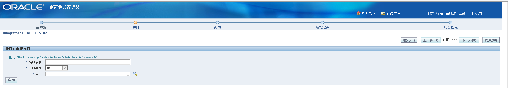
Oracle EBS ADI development steps
![[model distillation] tinybert: distilling Bert for natural language understanding](/img/c1/e1c1a3cf039c4df1b59ef4b4afbcb2.png)
[model distillation] tinybert: distilling Bert for natural language understanding

如何高效开发一款微信小程序
论文写作tip2

《Handwritten Mathematical Expression Recognition with Bidirectionally Trained Transformer》论文翻译
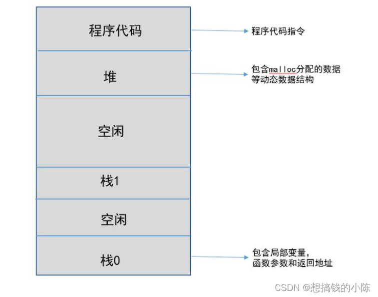
程序的内存模型

Implementation of purchase, sales and inventory system with ssm+mysql
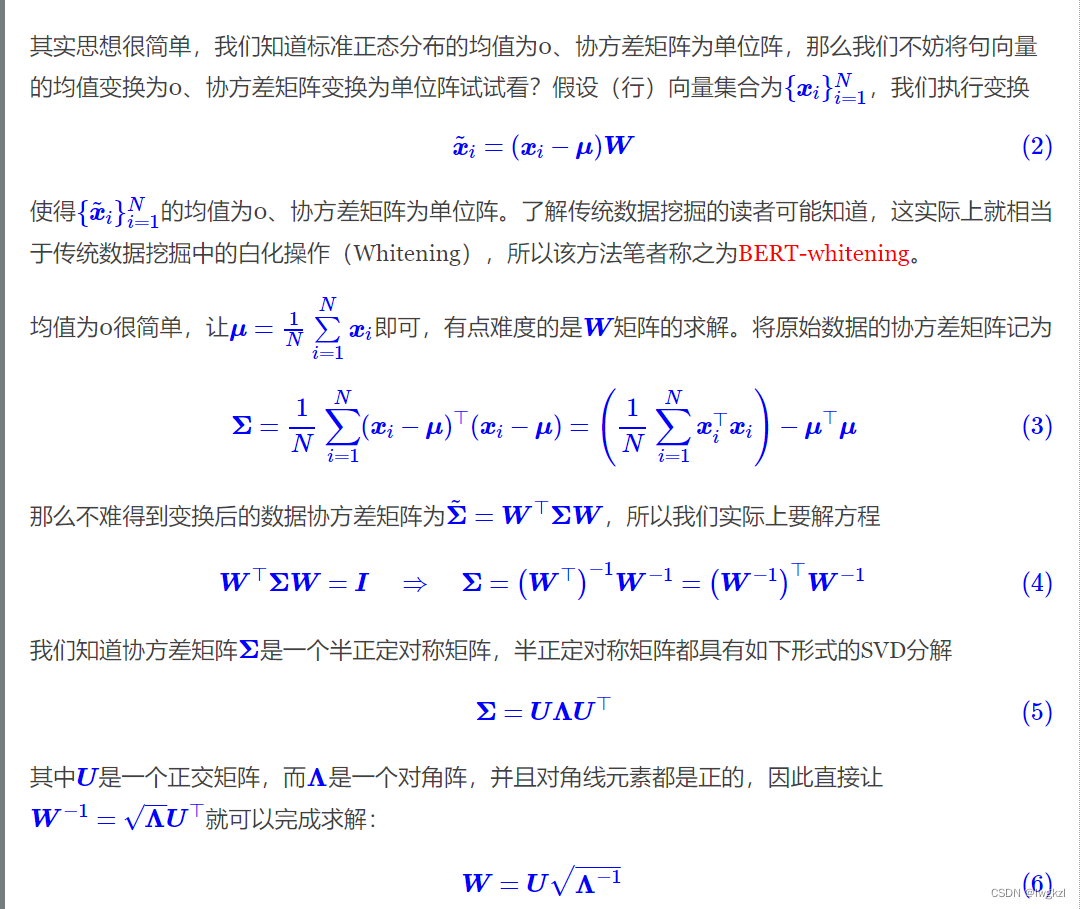
【调参Tricks】WhiteningBERT: An Easy Unsupervised Sentence Embedding Approach
随机推荐
Conda 创建,复制,分享虚拟环境
一份Slide两张表格带你快速了解目标检测
[introduction to information retrieval] Chapter II vocabulary dictionary and inverted record table
华为机试题-20190417
Pratique et réflexion sur l'entrepôt de données hors ligne et le développement Bi
架构设计三原则
Two dimensional array de duplication in PHP
離線數倉和bi開發的實踐和思考
TimeCLR: A self-supervised contrastive learning framework for univariate time series representation
CRP implementation methodology
华为机试题
Get the uppercase initials of Chinese Pinyin in PHP
Module not found: Error: Can't resolve './$$_gendir/app/app.module.ngfactory'
[torch] some ideas to solve the problem that the tensor parameters have gradients and the weight is not updated
[torch] the most concise logging User Guide
view的绘制机制(三)
win10解决IE浏览器安装不上的问题
Oracle EBS DataGuard setup
【Ranking】Pre-trained Language Model based Ranking in Baidu Search
Implement interface Iterable & lt; T&gt;