当前位置:网站首页>[CV] Wu Enda machine learning course notes | Chapter 9
[CV] Wu Enda machine learning course notes | Chapter 9
2022-07-04 08:13:00 【Fannnnf】
If there is no special explanation in this series of articles , The text explains the picture above the text
machine learning | Coursera
Wu Enda machine learning series _bilibili
Catalog
9 neural network :Learning
9-1 Cost function applied to neural network
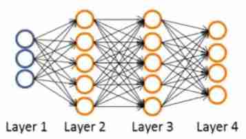
- use L L L Represents the total number of layers of the neural network (Layers)
- use s l s_l sl It means the first one l l l Layer unit ( Neuron ) The number of ( The bias unit is not included )
- h Θ ( x ) ∈ R K h_\Theta(x)\in\mathbb{R}^K hΘ(x)∈RK( h Θ ( x ) h_\Theta(x) hΘ(x) by K K K Dimension vector , Common to the output layer of neural network K K K Neurons , That is to say K K K Outputs )
- ( h Θ ( x ) ) i = i t h o u t p u t (h_\Theta(x))_i=i^{th} output (hΘ(x))i=ithoutput( ( h Θ ( x ) ) i (h_\Theta(x))_i (hΘ(x))i It means the first one i i i Outputs )
The cost function applied to neural networks is :
J ( Θ ) = − 1 m [ ∑ i = 1 m ∑ k = 1 K y ( i ) l o g ( h Θ ( x ( i ) ) ) k + ( 1 − y k ( i ) ) l o g ( 1 − ( h Θ ( x ( i ) ) ) k ) ] + λ 2 m ∑ l = 1 L − 1 ∑ i = 1 s l ∑ j = 1 s l + 1 ( Θ j i ( l ) ) 2 J(\Theta)=-\frac{1}{m}\left[\sum_{i=1}^m\sum_{k=1}^Ky^{(i)}log(h_\Theta(x^{(i)}))_k+(1-y_k^{(i)})log(1-(h_\Theta(x^{(i)}))_k)\right] +\frac{λ}{2m}\sum_{l=1}^{L-1}\sum_{i=1}^{s_l}\sum_{j=1}^{s_{l+1}}(\Theta_{ji}^{(l)})^2 J(Θ)=−m1[i=1∑mk=1∑Ky(i)log(hΘ(x(i)))k+(1−yk(i))log(1−(hΘ(x(i)))k)]+2mλl=1∑L−1i=1∑slj=1∑sl+1(Θji(l))2
- In the second item ∑ i = 1 s l ∑ j = 1 s l + 1 \sum_{i=1}^{s_l}\sum_{j=1}^{s_{l+1}} ∑i=1sl∑j=1sl+1 It means to be s l + 1 s_{l+1} sl+1 That's ok s l s_l sl Columns of the matrix Θ j i ( l ) \Theta_{ji}^{(l)} Θji(l) Add up each element in
- In the second item ∑ l = 1 L − 1 \sum_{l=1}^{L-1} ∑l=1L−1 It refers to summing the matrices of the input layer and the hidden layer
9-2 Back propagation algorithm
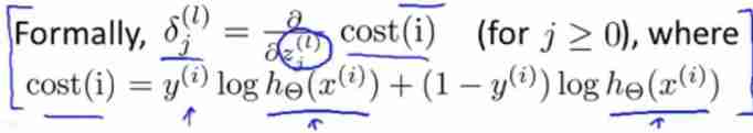
- δ j ( l ) \delta_j^{(l)} δj(l) It is defined as the first l l l Layer j j j Deviation of neurons (“error”)
Take the four layer neural network in the above figure as an example - δ j ( 4 ) = a j ( 4 ) − y j \delta_j^{(4)}=a_j^{(4)}-y_j δj(4)=aj(4)−yj( y j y_j yj Refers to the first j j j Output values in the data set , a j ( 4 ) a_j^{(4)} aj(4) It refers to the second of neural network j j j Outputs , a j ( 4 ) a_j^{(4)} aj(4) It can also be expressed as ( h Θ ( x ) ) j (h_\Theta(x))_j (hΘ(x))j)
- The above formula can be expressed as δ ( 4 ) = a ( 4 ) − y \delta^{(4)}=a^{(4)}-y δ(4)=a(4)−y, It can also be expressed as δ ( 4 ) = h Θ ( x ) − y \delta^{(4)}=h_\Theta(x)-y δ(4)=hΘ(x)−y
- δ ( 3 ) = ( Θ ( 3 ) ) T δ ( 4 ) ⋅ g ′ ( z ( 3 ) ) \delta^{(3)}=(\Theta^{(3)})^T\delta^{(4)}\cdot g^{\prime}(z^{(3)}) δ(3)=(Θ(3))Tδ(4)⋅g′(z(3))
among g ′ ( z ( 3 ) ) = a ( 3 ) ⋅ ( 1 − a ( 3 ) ) g^{\prime}(z^{(3)})=a^{(3)}\cdot (1-a^{(3)}) g′(z(3))=a(3)⋅(1−a(3)) - δ ( 2 ) = ( Θ ( 2 ) ) T δ ( 3 ) ⋅ g ′ ( z ( 2 ) ) \delta^{(2)}=(\Theta^{(2)})^T\delta^{(3)}\cdot g^{\prime}(z^{(2)}) δ(2)=(Θ(2))Tδ(3)⋅g′(z(2))
among g ′ ( z ( 2 ) ) = a ( 2 ) ⋅ ( 1 − a ( 2 ) ) g^{\prime}(z^{(2)})=a^{(2)}\cdot (1-a^{(2)}) g′(z(2))=a(2)⋅(1−a(2))
The result of dot multiplication is a number , The cross product is a vector
- ∂ ∂ Θ i j ( l ) J ( Θ ) = a j ( l ) δ i ( l + 1 ) \frac{\partial}{\partial \Theta_{ij}^{(l)}}J(\Theta)=a_j^{(l)}\delta_i^{(l+1)} ∂Θij(l)∂J(Θ)=aj(l)δi(l+1)
The regularization term is ignored here , The idea that λ = 0 \lambda=0 λ=0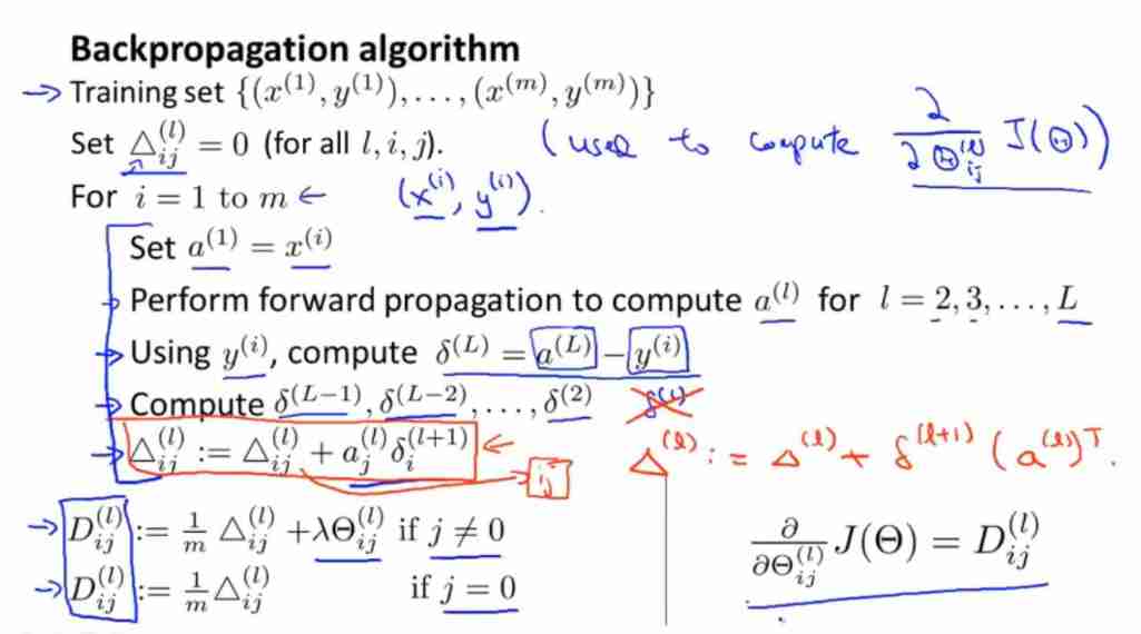
- The above figure is the flow of the back propagation algorithm , Finally, we can get ∂ ∂ Θ i j ( l ) J ( Θ ) = D i j ( l ) \frac{\partial}{\partial \Theta_{ij}^{(l)}}J(\Theta)=D^{(l)}_{ij} ∂Θij(l)∂J(Θ)=Dij(l), Then carry out gradient descent algorithm
9-3 Understand back propagation
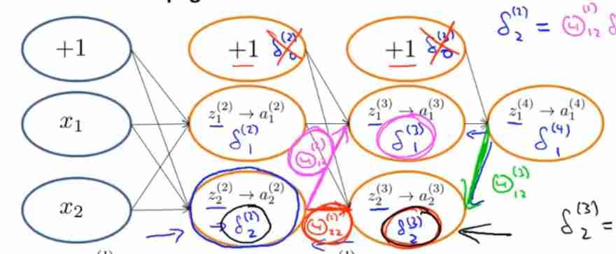
Take the neural network in the figure above as an example
- δ 2 ( 2 ) = Θ 12 ( 2 ) δ 1 ( 3 ) + Θ 22 ( 2 ) δ 2 ( 3 ) \delta_2^{(2)}=\Theta_{12}^{(2)}\delta_1^{(3)}+\Theta_{22}^{(2)}\delta_2^{(3)} δ2(2)=Θ12(2)δ1(3)+Θ22(2)δ2(3)
- δ 2 ( 3 ) = Θ 12 ( 3 ) δ 1 ( 4 ) \delta_2^{(3)}=\Theta_{12}^{(3)}\delta_1^{(4)} δ2(3)=Θ12(3)δ1(4)
9-4 Expand parameters
9-5 Gradient detection
To estimate the cost function J ( Θ ) J(\Theta) J(Θ) Upper point ( θ , J ( Θ ) ) (\theta,J(\Theta)) (θ,J(Θ)) Derivative at , Can use d d θ J ( θ ) ≈ J ( θ + ε ) − J ( θ − ε ) 2 ε ( ε = 1 0 − 4 by should ) \frac{\mathrm{d} }{\mathrm{d} \theta}J(\theta)\approx\frac{J(\theta+\varepsilon)-J(\theta-\varepsilon)}{2\varepsilon}(\varepsilon=10^{-4} It is advisable to ) dθdJ(θ)≈2εJ(θ+ε)−J(θ−ε)(ε=10−4 by should ) Obtain derivative 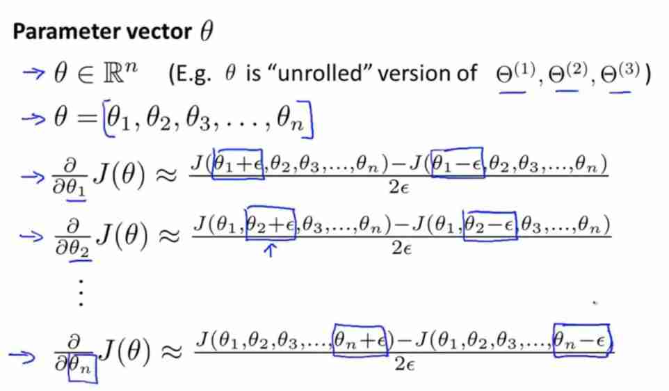
Expand into vectors , Pictured above
- θ \theta θ It's a n n n Dimension vector , It's a matrix Θ ( 1 ) , Θ ( 2 ) , Θ ( 3 ) , . . . \Theta^{(1)},\Theta^{(2)},\Theta^{(3)},... Θ(1),Θ(2),Θ(3),... Expansion of
- It can be estimated that ∂ ∂ θ n J ( θ ) \frac{\partial}{\partial \theta_{n}}J(\theta) ∂θn∂J(θ) Value
Compare the estimated partial derivative value with the partial derivative value obtained by back propagation , If the two values are very close , You can verify that the calculation is correct
Once it is determined that the value calculated by the back propagation algorithm is correct , You should turn off the gradient test algorithm
9-6 Random initialization
If at the beginning of the program Θ \Theta Θ All elements in are 0, It will cause multiple neurons to calculate the same characteristics , Leading to redundancy , This becomes a symmetric weight problem
So when initializing, make Θ i j ( l ) \Theta^{(l)}_{ij} Θij(l) be equal to [ − ϵ , ϵ ] [-\epsilon,\epsilon] [−ϵ,ϵ] A random value in
9-7 Review summary
Train a neural network :
1. Random an initial weight
2. Execute forward propagation algorithm , Get to all x ( i ) x^{(i)} x(i) Of h Θ ( x ( i ) ) h_\Theta(x^{(i)}) hΘ(x(i))
3. Computational cost function J ( Θ ) J(\Theta) J(Θ)
4. Execute back propagation algorithm , Calculation ∂ ∂ Θ j k ( l ) J ( Θ ) \frac{\partial}{\partial\Theta_{jk}^{(l)}}J(\Theta) ∂Θjk(l)∂J(Θ)
(get a ( l ) a^{(l)} a(l) and δ ( l ) \delta^{(l)} δ(l) for l = 2 , . . . , L l=2,...,L l=2,...,L)
5. Estimated by gradient test algorithm J ( Θ ) J(\Theta) J(Θ) Partial derivative of , Compare the estimated partial derivative value with the partial derivative value obtained by back propagation , If the two values are very close , It can be verified that the calculation result of the back propagation algorithm is correct ; After verification , Turn off the run Inspection Algorithm (disable gradient checking code)
6. Use gradient descent algorithm or other more advanced optimization methods , Combined with the back propagation calculation results , Get to make J ( Θ ) J(\Theta) J(Θ) The smallest parameter Θ \Theta Θ Value
边栏推荐
- R language uses cforest function in Party package to build random forest based on conditional inference trees, uses varimp function to check feature importance, and uses table function to calculate co
- 21个战略性目标实例,推动你的公司快速发展
- @Role of pathvariable annotation
- 墨者学院-Webmin未经身份验证的远程代码执行
- How to reset IntelliSense in vs Code- How to reset intellisense in VS Code?
- Comparison between applet framework and platform compilation
- BUUCTF(3)
- string. Format without decimal places will generate unexpected rounding - C #
- OKR vs. KPI figure out these two concepts at once!
- Leetcode (215) -- the kth largest element in the array
猜你喜欢
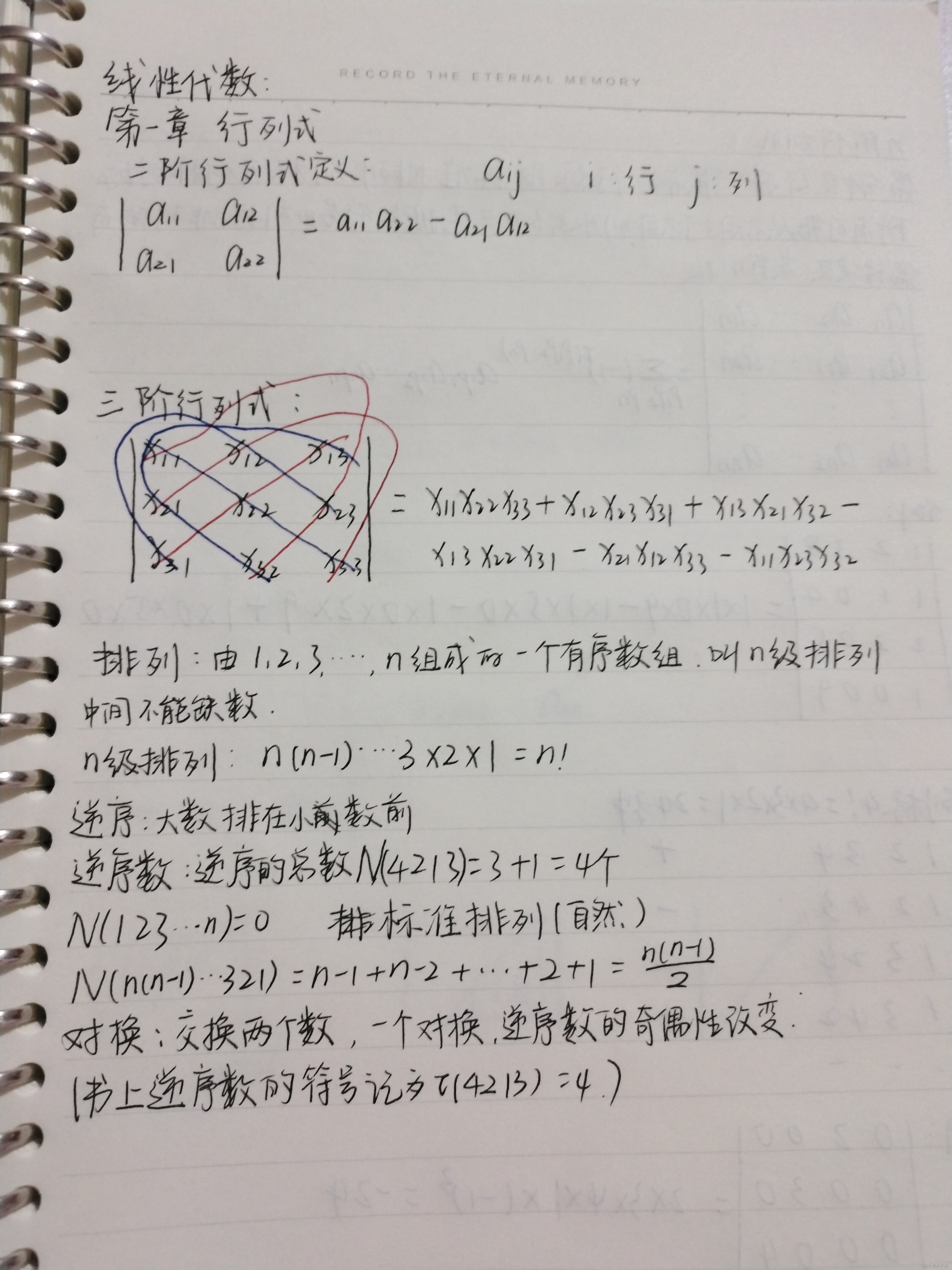
线性代数1.1
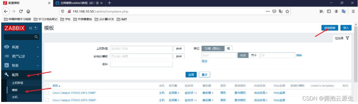
ZABBIX monitoring system custom monitoring content
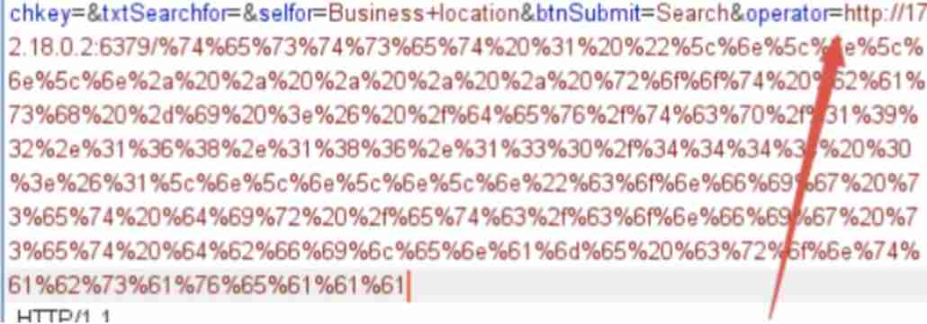
SSRF vulnerability exploitation - attack redis

Advanced MySQL: Basics (5-8 Lectures)
![Sports [running 01] a programmer's half horse challenge: preparation before running + adjustment during running + recovery after running (experience sharing)](/img/c8/39c394ca66348044834eb54c68c2a7.png)
Sports [running 01] a programmer's half horse challenge: preparation before running + adjustment during running + recovery after running (experience sharing)
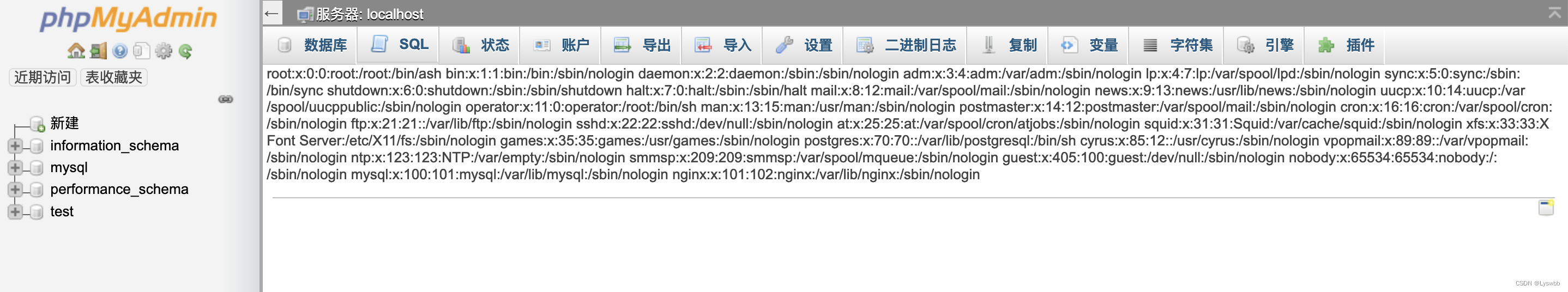
墨者学院-phpMyAdmin后台文件包含分析溯源
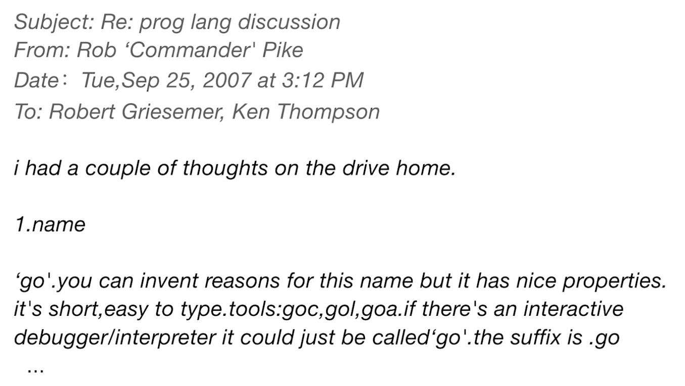
【Go基础】1 - Go Go Go
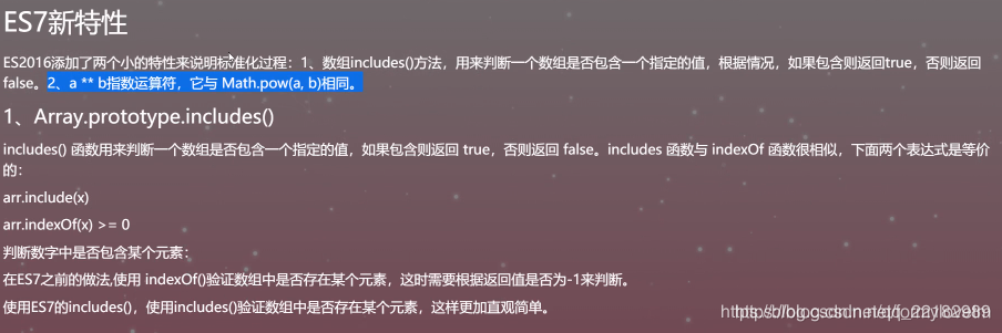
es6总结
论文学习——基于极值点特征的时间序列相似性查询方法
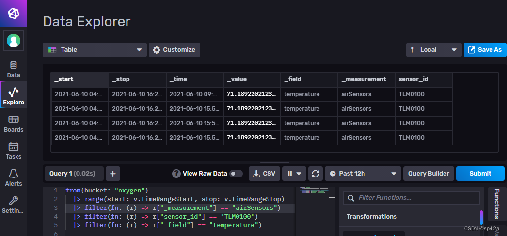
Preliminary study on temporal database incluxdb 2.2
随机推荐
Leetcode 146. LRU cache
Système de surveillance zabbix contenu de surveillance personnalisé
Mouse over to change the transparency of web page image
弈柯莱生物冲刺科创板:年营收3.3亿 弘晖基金与淡马锡是股东
Activiti常见操作数据表关系
猜数字游戏
Redis 哨兵机制
PHP session variable passed from form - PHP
ZABBIX 5.0 monitoring client
1. Getting started with QT
Oracle-存储过程与函数
Thesis learning -- time series similarity query method based on extreme point characteristics
Mysql database - function constraint multi table query transaction
【Go基础】1 - Go Go Go
Use preg_ Match extracts the string into the array between: & | people PHP
Set and modify the page address bar icon favicon ico
21个战略性目标实例,推动你的公司快速发展
Collections in Scala
DM8 database recovery based on point in time
Difference between static method and non static method (advantages / disadvantages)