当前位置:网站首页>Introduction to Robotics II. Forward kinematics, MDH method
Introduction to Robotics II. Forward kinematics, MDH method
2022-07-02 03:27:00 【RuiH. AI】
Introduction to Robotics Two 、 Forward kinematics
Preface
This chapter studies the forward kinematics of the manipulator ,MDH Law .
Joints and links
The joints joint, connecting rod link, It is the basic structure of the manipulator .
Joints include rotating joints and moving joints , Generally, there is only one degree of freedom .
One joint connects two adjacent connecting rods ,n Joint handle n+1 Connecting rods , have n A degree of freedom .
Number
Take the fixed base as the first 0 A connecting rod , The connecting rod at the end of the manipulator is used as the n A connecting rod .
Connecting rod parameters
Description of connecting rod
The length of the common vertical line between two adjacent joint axes , It is called the length of the connecting rod .
The angle formed between two adjacent joint axes , It is called the angle of the connecting rod .
Above picture , connecting rod i-1 The length of is its proximal joint axis i-1 With the distal joint axis i The length of the common vertical line between a i − 1 a_{i-1} ai−1
connecting rod i-1 The corner of is its proximal joint axis i-1 With the distal joint axis i Form an angle α i − 1 \alpha_{i-1} αi−1, As for the sign of angle , It can be determined when the coordinate system is established later .
Description of connecting rod connection
The distance between two adjacent connecting rods , It is called connecting rod offset .
The included angle of rotation of two adjacent connecting rods around the common joint axis , It is called joint angle .
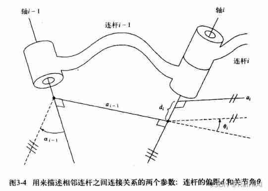
Above picture , The joints i It's the connecting rod i-1 And connecting rod i The common joint of .
Because the actual connecting rod is bent , The common vertical line segment a i − 1 a_{i-1} ai−1 and a i a_i ai As a straight connecting rod instead of a curved connecting rod i-1,i.
Straight link i-1,i The distance between them is the joint i Connecting rod offset d i d_i di
Straight link i-1 Along the joint axis i Rotate to the straight link i The angle of is the joint angle θ i \theta_i θi
Joint variables
A connecting rod can use the upper connecting rod length 、 Connecting rod angle 、 Connecting rod offset 、 Four parameters of joint angle are determined .
For rotating joints , The joint angle is variable , The other three parameters remain unchanged .
For moving joints , The connecting rod offset is variable , The other three parameters remain unchanged .
Variable parameters are called joint variables .
The connecting rod coordinate system
The connecting rod coordinate system is used to describe the relative position relationship between adjacent connecting rods .
The number of the connecting rod coordinate system is the same as that of the connecting rod , be called { i } \{i\} { i}.
The coordinate system of the intermediate connecting rod is established
For connecting rod i Set up a coordinate system :
With joint axis i As Z Axis , With connecting rod i And Z Axis As origin , With connecting rod i As X Axis Point to the joint axis i+1, The right-hand rule determines Y Axis .
exception : If the connecting rod i The length of a i = 0 a_i=0 ai=0( At this time, the connecting rod i,i+1 Of Z Axis The intersection ), Take the intersection as origin , With Two Z The plane of the axis The vertical line of X Axis , There are two choices of direction , and α i \alpha_i αi The symbol of is composed of X Axis Direction determines .
The establishment of each coordinate axis should meet the right-hand rule .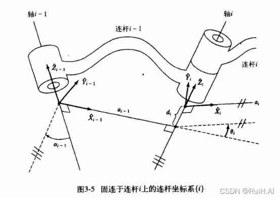
Above picture , The coordinate system can be established in this order :
First find all the joint axes i-1,i
Then determine the coordinate system { i − 1 } \{i-1\} { i−1}, Take the joint axis as Z ^ i − 1 \hat Z_{i-1} Z^i−1, Straight link i-1 As X ^ i − 1 \hat X_{i-1} X^i−1, Then the right hand rule determines Y ^ i − 1 \hat Y_{i-1} Y^i−1.
Then determine the coordinate system { i } \{i\} { i}.
Establish the coordinate system of the head and tail connecting rods
For the head and tail connecting rods 0,n, There is a special way to build a department .
Head coordinate system
Coordinate system { 0 } \{0\} { 0} On the base , Generally used as a reference system .
The first joint variable is 0 when , Specify the coordinate system { 0 } \{0\} { 0} On { 1 } \{1\} { 1} coincidence .
When the first joint is a rotating joint , d 1 = 0 d_1=0 d1=0; The first joint is the mobile joint , θ 1 = 0 \theta_1=0 θ1=0
Tail coordinate system
Coordinate system { n } \{n\} { n} Origin and x Axis The direction can be arbitrarily selected , But try to make the connecting rod parameters 0.
Connecting rod parameters and connecting rod coordinate system
Follow the above method of building a department , The connecting rod parameters can be redefined :
- a i a_i ai Connecting rod length : Along the X ^ i \hat X_i X^i, from Z ^ i \hat Z_i Z^i Move to Z ^ i + 1 \hat Z_{i+1} Z^i+1 Distance of
- α i \alpha_i αi Connecting rod torsion angle : Around the X ^ i \hat X_i X^i Axis , hold Z ^ i \hat Z_i Z^i Rotate to Z ^ i + 1 \hat Z_{i+1} Z^i+1 The angle of
- d i d_i di Connecting rod offset : Along the Z ^ i \hat Z_i Z^i, from X ^ i − 1 \hat X_{i-1} X^i−1 Move to X ^ i 1 \hat X_{i1} X^i1 Distance of
- θ i \theta_i θi Joint angle : Around the Z ^ i \hat Z_i Z^i Axis , hold X ^ i − 1 \hat X_{i-1} X^i−1 Rotate to X ^ i \hat X_{i} X^i The angle of
Set up a i > 0 a_i>0 ai>0, Other parameters can be positive or negative .
The above method of establishing the connecting rod coordinate system and connecting rod parameters is called MDH Law (Modified Denavit–Hartenberg).
DH The coordinate system established by the method is not unique .
Connecting rod change
Connecting rod parameters can be used to calculate the relative pose between adjacent rods .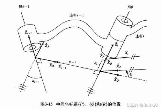
Above picture , Consider the coordinate system { i − 1 } , { i } \{i-1\},\{i\} { i−1},{ i} The transformation between i − 1 i T ^i_{i-1}T i−1iT, Establish an intermediate coordinate system { P } , { Q } , { R } \{P\},\{Q\},\{R\} { P},{ Q},{ R}, Then there are :
i i − 1 T = R i − 1 T Q R T P Q T i P T ^{i-1}_iT = \ ^{i-1}_RT \ ^R_{Q}T \ ^Q_PT \ ^P_{i}T ii−1T= Ri−1T QRT PQT iPT
The transformation above , It can be seen as putting X ^ i \hat X_i X^i Transformation for X ^ i − 1 \hat X_{i-1} X^i−1, Then there are :
i i − 1 T = R X ( α i − 1 ) D X ( a i − 1 ) R Z ( θ i ) D Z ( d i ) ^{i-1}_iT = R_X(\alpha_{i-1})D_X(a_{i-1})R_Z(\theta_i)D_Z(d_i) ii−1T=RX(αi−1)DX(ai−1)RZ(θi)DZ(di)
Or write out the transformation of each intermediate coordinate system :
i P T = [ 1 0 0 0 0 1 0 0 0 0 1 d i 0 0 0 1 ] P Q T = [ cos θ 1 − sin θ 1 0 0 sin θ 1 cos θ 1 0 0 0 0 1 0 0 0 0 1 ] Q R T = [ 1 0 0 0 0 1 0 a i − 1 0 0 1 0 0 0 0 1 ] R i − 1 T = [ 1 0 0 0 0 cos α i − 1 − sin α i − 1 0 0 sin α i − 1 cos α i − 1 0 0 0 0 1 ] ^P_iT = \begin{bmatrix} 1 & 0 & 0 & 0 \\ 0 & 1 & 0 & 0 \\ 0 & 0 & 1 & d_i \\ 0 & 0 & 0 & 1 \\ \end{bmatrix} \\ \quad \\ \ ^Q_PT = \begin{bmatrix} \cos \theta_1 & -\sin \theta_1 & 0 & 0 \\ \sin \theta_1 & \cos \theta_1 & 0 & 0 \\ 0 & 0 & 1 &0 \\ 0 & 0 & 0 & 1 \\ \end{bmatrix} \\ \quad \\ \ ^R_QT = \begin{bmatrix} 1 & 0 & 0 & 0 \\ 0 & 1 & 0 & a_{i-1} \\ 0 & 0 & 1 & 0 \\ 0 & 0 & 0 & 1 \\ \end{bmatrix} \\ \quad \\ \ ^{i-1}_RT = \begin{bmatrix} 1 & 0 & 0 & 0 \\ 0 & \cos \alpha_{i-1} & -\sin \alpha_{i-1} & 0 \\ 0 & \sin \alpha_{i-1} & \cos \alpha_{i-1} & 0 \\ 0 & 0 & 0 & 1 \\ \end{bmatrix} \\ \quad \\ iPT=⎣⎢⎢⎡10000100001000di1⎦⎥⎥⎤ PQT=⎣⎢⎢⎡cosθ1sinθ100−sinθ1cosθ10000100001⎦⎥⎥⎤ QRT=⎣⎢⎢⎡1000010000100ai−101⎦⎥⎥⎤ Ri−1T=⎣⎢⎢⎡10000cosαi−1sinαi−100−sinαi−1cosαi−100001⎦⎥⎥⎤
obtain i i − 1 T ^{i-1}_iT ii−1T The general form of :
MDH Method use steps
- Find all joint axes ;
- Establish the coordinate system of the intermediate connecting rod in sequence ;
- Determine the head and tail coordinate system ;
- Write DH Parameters ;
- Calculate the forward kinematics matrix .
Postscript
This article is about forward kinematics in robotics , It's using MDH Law .
There will be Matlab Example programming .
边栏推荐
- 焱融看 | 混合云时代下,如何制定多云策略
- /silicosis/geo/GSE184854_ scRNA-seq_ mouse_ lung_ ccr2/GSE184854_ RAW/GSM5598265_ matrix_ inflection_ demult
- "Analysis of 43 cases of MATLAB neural network": Chapter 41 implementation of customized neural network -- personalized modeling and Simulation of neural network
- In the era of programmers' introspection, five-year-old programmers are afraid to go out for interviews
- OSPF LSA message parsing (under update)
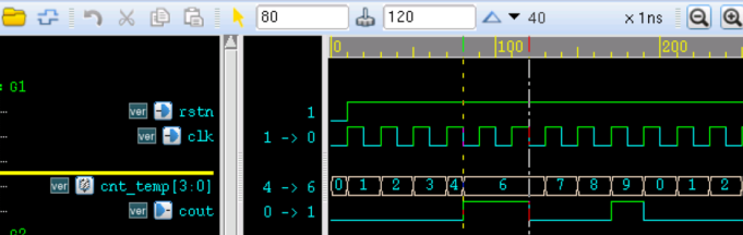
- Verilog 避免 Latch
- Verilog 过程赋值 区别 详解
- 终日乾乾,夕惕若厉
- [C Advanced] brother Peng takes you to play with strings and memory functions
- Continuous assignment of Verilog procedure
猜你喜欢
Halcon image rectification
JS introduction < 1 >
C reflection practice
JS <2>
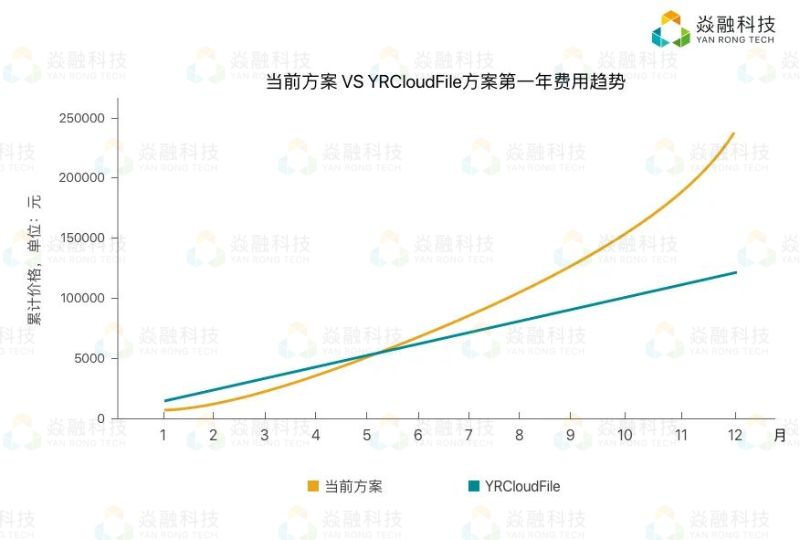
Yan Rong looks at how to formulate a multi cloud strategy in the era of hybrid cloud

Analyse de 43 cas de réseaux neuronaux MATLAB: Chapitre 42 opérations parallèles et réseaux neuronaux - - opérations parallèles de réseaux neuronaux basées sur CPU / GPU
Knowing things by learning | self supervised learning helps improve the effect of content risk control
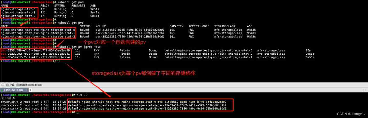
Kubernetes cluster storageclass persistent storage resource core concept and use
Continuous assignment of Verilog procedure
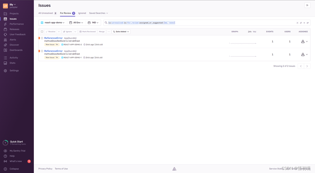
Sentry experience and architecture, a fledgling monitoring product with a market value of $100million
随机推荐
< job search> process and signal
C reflection practice
Generate random numbers that obey normal distribution
[HCIA continuous update] working principle of OSPF Protocol
QT environment generates dump to solve abnormal crash
The page in H5 shows hidden execution events
Docker installs canal and MySQL for simple testing and implementation of redis and MySQL cache consistency
Load different fonts in QML
Grpc快速实践
Pycharm2021 delete the package warehouse list you added
Knowing things by learning | self supervised learning helps improve the effect of content risk control
Go execute shell command
Kotlin 基础学习13
Calculation of page table size of level 2, level 3 and level 4 in protection mode (4k=4*2^10)
Sentry experience and architecture, a fledgling monitoring product with a market value of $100million
Uniapp uses canvas to generate posters and save them locally
流线线使用阻塞还是非阻塞
Exchange rate query interface
Getting started with MQ
Xlwings drawing