当前位置:网站首页>"Analysis of 43 cases of MATLAB neural network": Chapter 41 implementation of customized neural network -- personalized modeling and Simulation of neural network
"Analysis of 43 cases of MATLAB neural network": Chapter 41 implementation of customized neural network -- personalized modeling and Simulation of neural network
2022-07-02 03:24:00 【mozun2020】
《MATLAB neural network 43 A case study 》: The first 41 Chapter Implementation of customized neural network —— Personalized modeling and Simulation of Neural Networks
1. Preface
《MATLAB neural network 43 A case study 》 yes MATLAB Technology Forum (www.matlabsky.com) planning , Led by teacher wangxiaochuan ,2013 Beijing University of Aeronautics and Astronautics Press MATLAB A book for tools MATLAB Example teaching books , Is in 《MATLAB neural network 30 A case study 》 On the basis of modification 、 Complementary , Adhering to “ Theoretical explanation — case analysis — Application extension ” This feature , Help readers to be more intuitive 、 Learn neural networks vividly .
《MATLAB neural network 43 A case study 》 share 43 Chapter , The content covers common neural networks (BP、RBF、SOM、Hopfield、Elman、LVQ、Kohonen、GRNN、NARX etc. ) And related intelligent algorithms (SVM、 Decision tree 、 Random forests 、 Extreme learning machine, etc ). meanwhile , Some chapters also cover common optimization algorithms ( Genetic algorithm (ga) 、 Ant colony algorithm, etc ) And neural network . Besides ,《MATLAB neural network 43 A case study 》 It also introduces MATLAB R2012b New functions and features of neural network toolbox in , Such as neural network parallel computing 、 Custom neural networks 、 Efficient programming of neural network, etc .
In recent years, with the rise of artificial intelligence research , The related direction of neural network has also ushered in another upsurge of research , Because of its outstanding performance in the field of signal processing , The neural network method is also being applied to various applications in the direction of speech and image , This paper combines the cases in the book , It is simulated and realized , It's a relearning , I hope I can review the old and know the new , Strengthen and improve my understanding and practice of the application of neural network in various fields . I just started this book on catching more fish , Let's start the simulation example , Mainly to introduce the source code application examples in each chapter , This paper is mainly based on MATLAB2015b(32 position ) Platform simulation implementation , This is the implementation example of customized neural network in Chapter 41 of this book , Don't talk much , Start !
2. MATLAB Simulation example
open MATLAB, Click on “ Home page ”, Click on “ open ”, Find the sample file 
Choose chapter41.m, Click on “ open ”
chapter41.m Source code is as follows :
%%%%%%%%%%%%%%%%%%%%%%%%%%%%%%%%%%%%%%%%%%%%%%%%%%%%
% function : Implementation of customized neural network - Personalized modeling and Simulation of Neural Networks
% Environmental Science :Win7,Matlab2015b
%Modi: C.S
% Time :2022-06-21
%%%%%%%%%%%%%%%%%%%%%%%%%%%%%%%%%%%%%%%%%%%%%%%%%%%%
%% Matlab neural network 43 A case study
% Implementation of customized neural network - Personalized modeling and Simulation of Neural Networks
% by Wang Xiao Chuan (@ Wang Xiao Chuan _matlab)
% http://www.matlabsky.com
% Email:[email protected]163.com
% http://weibo.com/hgsz2003
%% Clear environment variables
clear all
clc
warning off
tic
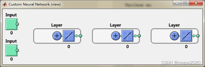
%% Build a “ empty ” neural network
net = network
%% Input and network layer definition
net.numInputs = 2;
net.numLayers = 3;
%% Use view(net) Observe the neural network structure .
view(net)
% At this time, the neural network has two inputs , Three neuron layers . But please pay attention to :net.numInputs The settings are
% The number of inputs of neural network , The dimension of each input is determined by net.inputs{
i}.size control .
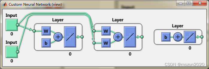
%% Threshold connection definition
net.biasConnect(1) = 1;
net.biasConnect(3) = 1;
% Or use net.biasConnect = [1; 0; 1];
view(net)
%% Input and layer connection definitions
net.inputConnect(1,1) = 1;
net.inputConnect(2,1) = 1;
net.inputConnect(2,2) = 1;
% Or use net.inputConnect = [1 0; 1 1; 0 0];
view(net)
net.layerConnect = [0 0 0; 0 0 0; 1 1 1];
view(net)
%% Output connection settings
net.outputConnect = [0 1 1];
view(net)
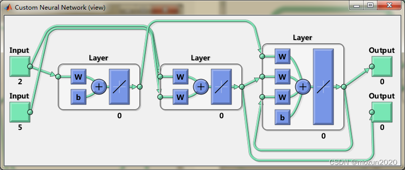
%% Enter Settings
net.inputs
net.inputs{
1}
net.inputs{
1}.processFcns = {
'removeconstantrows','mapminmax'};
net.inputs{
2}.size = 5;
net.inputs{
1}.exampleInput = [0 10 5; 0 3 10];
view(net)
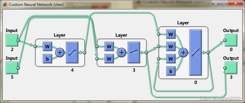
%% Layer Settings
net.layers{
1}
% Set the number of neurons in the first layer of the neural network to 4 individual , Its transfer function is set to “tansig” and
% Set its initialization function to Nguyen-Widrow function .
net.layers{
1}.size = 4;
net.layers{
1}.transferFcn = 'tansig';
net.layers{
1}.initFcn = 'initnw';
% Set the number of neurons in the second layer to 3 individual , Its transfer function is set to “logsig”, And use “initnw” initialization .
net.layers{
2}.size = 3;
net.layers{
2}.transferFcn = 'logsig';
net.layers{
2}.initFcn = 'initnw';
% Set the initialization function of the third layer to “initnw”
net.layers{
3}.initFcn = 'initnw';
view(net)
%% Output Settings
net.outputs
net.outputs{
2}
%% threshold , Input weight and layer weight settings
net.biases
net.biases{
1}
net.inputWeights
net.layerWeights
%% Set the delay of some weights of the neural network
net.inputWeights{
2,1}.delays = [0 1];
net.inputWeights{
2,2}.delays = 1;
net.layerWeights{
3,3}.delays = 1;
%% Network function settings
% Set the neural network initialization to “initlay”, In this way, the neural network can follow
% The layer initialization function we set “ initnw” namely Nguyen-Widrow To initialize .
net.initFcn = 'initlay';
% Set the error of neural network to “mse”(mean squared error), At the same time, the training function of neural network
% Set to “trainlm”Levenberg-Marquardt backpropagation).
net.performFcn = 'mse';
net.trainFcn = 'trainlm';
% In order to make the neural network can randomly divide the training data set , We can divideFcn Set to “dividerand”.
net.divideFcn = 'dividerand';
% take plot functions Set to :“plotperform”,“plottrainstate”
net.plotFcns = {
'plotperform','plottrainstate'};
%% Weight threshold size setting
net.IW{
1,1}, net.IW{
2,1}, net.IW{
2,2}
net.LW{
3,1}, net.LW{
3,2}, net.LW{
3,3}
net.b{
1}, net.b{
3}
%% Neural network initialization
net = init(net);
net.IW{
1,1}
%% Neural network training
X = {
[0; 0] [2; 0.5]; [2; -2; 1; 0; 1] [-1; -1; 1; 0; 1]};
T = {
[1; 1; 1] [0; 0; 0]; 1 -1};
Y = sim(net,X)
%% Training parameters of neural network
net.trainParam
%% Training network
net = train(net,X,T);
%% Simulation to check whether the neural network is normal .
Y = sim(net,X)
toc
Add completed , Click on “ function ”, Start emulating , The output simulation results are as follows :
net =

    Neural Network

              name: 'Custom Neural Network'
          userdata: (your custom info)

    dimensions:

         numInputs: 0
         numLayers: 0
        numOutputs: 0
    numInputDelays: 0
    numLayerDelays: 0
 numFeedbackDelays: 0
 numWeightElements: 0
        sampleTime: 1

    connections:

       biasConnect: []
      inputConnect: []
      layerConnect: []
     outputConnect: []

    subobjects:

            inputs: {
    0x1 cell array of 0 inputs}
            layers: {
    0x1 cell array of 0 layers}
           outputs: {
    1x0 cell array of 0 outputs}
            biases: {
    0x1 cell array of 0 biases}
      inputWeights: {
    0x0 cell array of 0 weights}
      layerWeights: {
    0x0 cell array of 0 weights}

    functions:

          adaptFcn: (none)
        adaptParam: (none)
          derivFcn: 'defaultderiv'
         divideFcn: (none)
       divideParam: (none)
        divideMode: 'sample'
           initFcn: 'initlay'
        performFcn: 'mse'
      performParam: .regularization, .normalization
          plotFcns: {
    }
        plotParams: {
    1x0 cell array of 0 params}
          trainFcn: (none)
        trainParam: (none)

    weight and bias values:

                IW: {
    0x0 cell} containing 0 input weight matrices
                LW: {
    0x0 cell} containing 0 layer weight matrices
                 b: {
    0x1 cell} containing 0 bias vectors

    methods:

             adapt: Learn while in continuous use
         configure: Configure inputs & outputs
            gensim: Generate Simulink model
              init: Initialize weights & biases
           perform: Calculate performance
               sim: Evaluate network outputs given inputs
             train: Train network with examples
              view: View diagram
       unconfigure: Unconfigure inputs & outputs


ans =

    [1x1 nnetInput]
    [1x1 nnetInput]


ans =

    Neural Network Input

              name: 'Input'
    feedbackOutput: []
       processFcns: {
    }
     processParams: {
    1x0 cell array of 0 params}
   processSettings: {
    0x0 cell array of 0 settings}
    processedRange: []
     processedSize: 0
             range: []
              size: 0
          userdata: (your custom info)


ans =

    Neural Network Layer

              name: 'Layer'
        dimensions: 0
       distanceFcn: (none)
     distanceParam: (none)
         distances: []
           initFcn: 'initwb'
       netInputFcn: 'netsum'
     netInputParam: (none)
         positions: []
             range: []
              size: 0
       topologyFcn: (none)
       transferFcn: 'purelin'
     transferParam: (none)
          userdata: (your custom info)


ans =

    []    [1x1 nnetOutput]    [1x1 nnetOutput]


ans =

    Neural Network Output

              name: 'Output'
     feedbackInput: []
     feedbackDelay: 0
      feedbackMode: 'none'
       processFcns: {
    }
     processParams: {
    1x0 cell array of 0 params}
   processSettings: {
    0x0 cell array of 0 settings}
    processedRange: [3x2 double]
     processedSize: 3
             range: [3x2 double]
              size: 3
          userdata: (your custom info)


ans =

    [1x1 nnetBias]
    []
    [1x1 nnetBias]


ans =

    Neural Network Bias

           initFcn: (none)
             learn: true
          learnFcn: (none)
        learnParam: (none)
              size: 4
          userdata: (your custom info)


ans =

    [1x1 nnetWeight]                  []
    [1x1 nnetWeight]    [1x1 nnetWeight]
                  []                  []


ans =

                  []                  []                  []
                  []                  []                  []
    [1x1 nnetWeight]    [1x1 nnetWeight]    [1x1 nnetWeight]


ans =

     0     0
     0     0
     0     0
     0     0


ans =

     0     0     0     0
     0     0     0     0
     0     0     0     0


ans =

     0     0     0     0     0
     0     0     0     0     0
     0     0     0     0     0


ans =

    Empty matrix : 0×4


ans =

    Empty matrix : 0×3


ans =

     []


ans =

     0
     0
     0
     0


ans =

    Empty matrix : 0×1


ans =

    1.9468    2.0124
    2.3881   -1.4619
   -1.7285    2.2028
   -0.2749    2.7865


Y =

    [3x1 double]    [3x1 double]
    [0x1 double]    [0x1 double]


ans =


    Function Parameters for 'trainlm'

    Show Training Window Feedback   showWindow: true
    Show Command Line Feedback showCommandLine: false
    Command Line Frequency                show: 25
    Maximum Epochs                      epochs: 1000
    Maximum Training Time                 time: Inf
    Performance Goal                      goal: 0
    Minimum Gradient                  min_grad: 1e-07
    Maximum Validation Checks         max_fail: 6
    Mu                                      mu: 0.001
    Mu Decrease Ratio                   mu_dec: 0.1
    Mu Increase Ratio                   mu_inc: 10
    Maximum mu                          mu_max: 10000000000


Y =

    [3x1 double]    [3x1 double]
    [    1.0000]    [   -1.0000]

 Time has passed  3.932652  second .


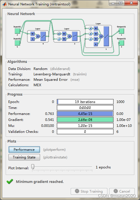
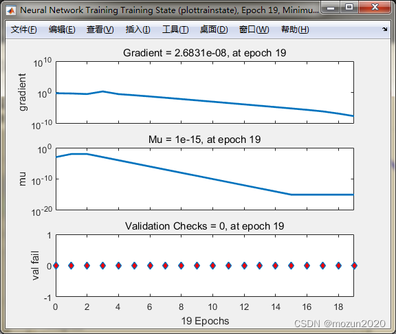
In turn, click Plots Medium Performance,Training State The following figure is available :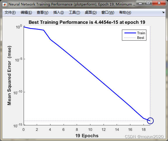
3. Summary
This chapter introduces the method of customizing neural network , Including how to set up the network , How to link the network , And through input and output , Connection threshold , Input connection , The connection of output, etc. shall be set accordingly , So as to get the neural network you need , Then import data for corresponding training , After obtaining the model, carry out the prediction test , A complete process of customizing neural network has been realized . Interested in the content of this chapter or want to fully learn and understand , It is suggested to study the contents of Chapter 41 in the book . Some of these knowledge points will be supplemented on the basis of their own understanding in the later stage , Welcome to study and exchange together .
边栏推荐
- Large screen visualization from bronze to the advanced king, you only need a "component reuse"!
- ORA-01547、ORA-01194、ORA-01110
- 命名块 verilog
- Kotlin 基础学习13
- C#联合halcon脱离halcon环境以及各种报错解决经历
- V-model of custom component
- GB/T-2423. XX environmental test documents, including the latest documents
- Competition and adventure burr
- 32, 64, 128 bit system
- Qualcomm platform wifi-- WPA_ supplicant issue
猜你喜欢
SAML2.0 笔记(一)
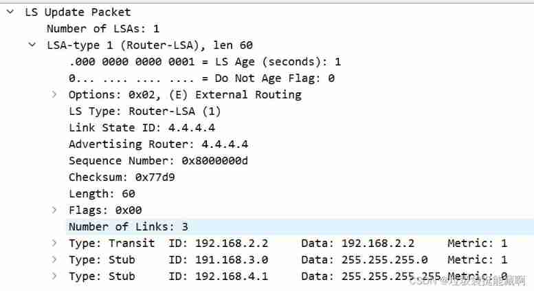
OSPF LSA message parsing (under update)

Named block Verilog

This article describes the step-by-step process of starting the NFT platform project
![[golang] leetcode intermediate bracket generation & Full Permutation](/img/93/ca38d97c721ccba2505052ef917788.jpg)
[golang] leetcode intermediate bracket generation & Full Permutation

Discrimination between sap Hana, s/4hana and SAP BTP

Download and use of the super perfect screenshot tool snipaste

The capacity is upgraded again, and the new 256gb large capacity specification of Lexar rexa 2000x memory card is added

Xiaomi, a young engineer, was just going to make soy sauce

How to establish its own NFT market platform in 2022
随机推荐
Download and use of the super perfect screenshot tool snipaste
JS <2>
Start a business
跟着CTF-wiki学pwn——ret2shellcode
Work hard all day long and be alert at sunset
Which of PMP and software has the highest gold content?
[JVM] detailed description of the process of creating objects
Redis set command line operation (intersection, union and difference, random reading, etc.)
verilog REG 寄存器、向量、整数、实数、时间寄存器
Generate random numbers that obey normal distribution
浅谈线程池相关配置
PHP array processing
Kotlin基础学习 14
初出茅庐市值1亿美金的监控产品Sentry体验与架构
《MATLAB 神经网络43个案例分析》:第42章 并行运算与神经网络——基于CPU/GPU的并行神经网络运算
/silicosis/geo/GSE184854_ scRNA-seq_ mouse_ lung_ ccr2/GSE184854_ RAW/GSM5598265_ matrix_ inflection_ demult
Framing in data transmission
2022 hoisting machinery command examination paper and summary of hoisting machinery command examination
PMP personal sprint preparation experience
PY3, PIP appears when installing the library, warning: ignoring invalid distribution -ip