当前位置:网站首页>Data classification: support vector machine
Data classification: support vector machine
2022-07-03 10:24:00 【Why】
One 、 Job requirements
- To write SVM Algorithmic program ( You can find the corresponding code from the network ), Platform self selection .
- Use SVM Algorithm , Three kernel functions are used to establish classification models for a given sample data set . The dimension in the data file “ type ” Is the type of identification .
- use 60% The data is the training set ,40% For test set , Accuracy of use 、 Test your results with sensitivity and specificity .
- Complete the excavation report .
Two 、 Data set pre analysis
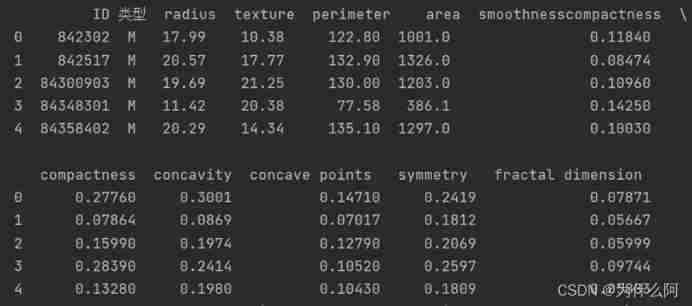
The first five items of the data set are shown
View the overall information of the dataset
The whole data set consists of 12 Column ,569 That's ok , No missing value , There is no need to deal with missing values .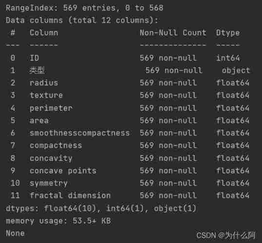
Comments for dataset columns
Include ID, Types and characteristics are 12 individual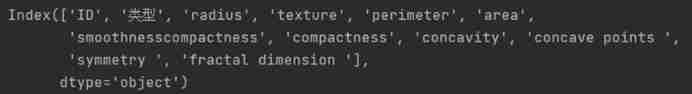
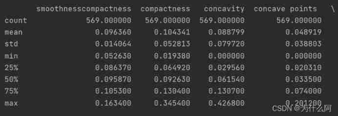
Check the average value of each characteristic of the data , variance , The most value , Index values such as quartile


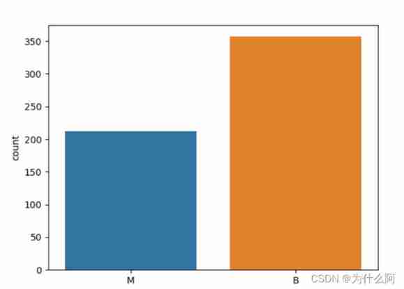
Visualization of the distribution of two types of data
3、 ... and 、 Data preprocessing
- feature selection
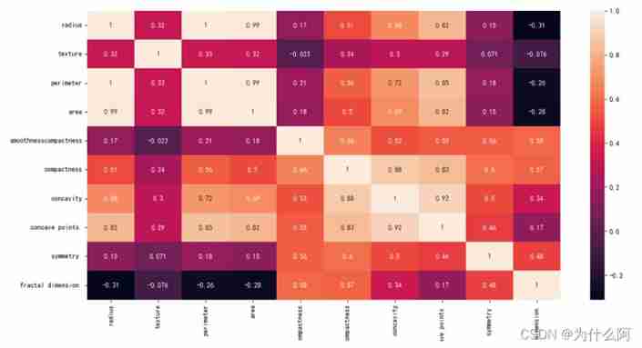
The correlation coefficient of the single variable itself on the diagonal of the thermodynamic diagram is 1, The lighter the color, the greater the correlation . It can be seen from the heat map radius_mean、perimeter_mean and area_mean Very relevant ,compactness_mean、concavity_mean、concave_points_mean this 3 Fields are also relevant , Therefore, you can choose radius_mean,perimeter_mean,area_mean,compactness_mean,concavity_mean,concave_points_mean These six features are the main features .
Four 、 Related knowledge
- SVM Kernel function
① Linear kernel function
Linear kernel function (Linear Kernel) In fact, it is linearly separable SVM, in other words , Linearly separable SVM Can be inseparable from linearity SVM Classed , The difference is only linear separability SVM Linear kernel function is used .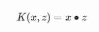
② Gaussian kernel
Gaussian kernel (Gaussian Kernel), stay SVM Also known as radial basis kernel function (Radial Basis Function,RBF), It is a nonlinear classification SVM The most popular kernel function , yes libsvm Default kernel function .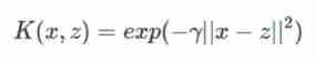
③ Sigmoid Kernel function
Sigmoid Kernel function (Sigmoid Kernel) It's also linear SVM One of the common kernel functions .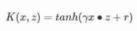
- SVM Performance metrics
① Confusion matrix
For the problem of two categories , The categories we care about are usually defined as positive classes , The other is called negative class . The confusion matrix consists of the following data :
True Positive ( real ,TP): The number of positive classes predicted as positive classes
True Negative ( True negative ,TN): The number of negative classes predicted as negative classes
False Positive( False positive ,FP): The number of negative classes predicted to be positive ( False positives )
False Negative( False negative ,FN): The number of positive classes predicted as negative classes ( Omission of )
| M | B | |
|---|---|---|
| F(False,0) | TN | FP |
| T(True,1) | FN | TP |
② Accuracy rate
Accuracy is the most common evaluation index , Predict the proportion of correct samples in all samples ; Generally speaking , The higher the accuracy, the better the classifier .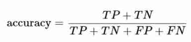
③ Sensitivity ( Recall rate )
Sensitivity represents the proportion of all positive examples in the sample that are identified , It measures the recognition ability of classifier to positive examples .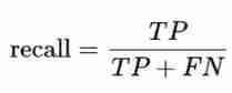
④ Special effect test ( Special effects )
The specific effect degree represents the proportion of all negative examples in the sample that are recognized , It measures the ability of the classifier to recognize negative examples .
5、 ... and 、 Outline design
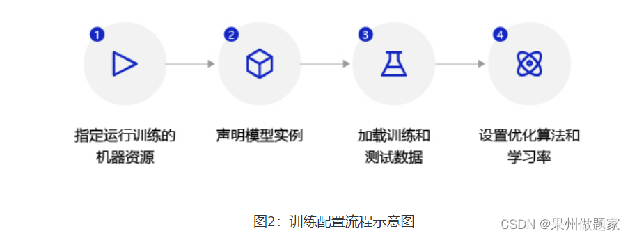
Outline design flow chart :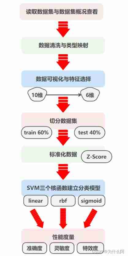
6、 ... and 、 Detailed design and core code
- Read datasets and view datasets overview
# Reading data sets
data = pd.read_excel(' Classification job data set .xlsx')
# Dataset view
print(data.info())
print(data.columns)
print(data.head(5))
print(data.describe())
- Data cleaning and type mapping
# Data cleaning
#“ID" Columns have no practical significance , Delete
data.drop('ID',axis = 1,inplace=True)
# Will be of type B,M use 0,1 Instead of
data[' type '] = data[' type '].map({
    'M':1,'B':0})
- Data visualization and feature selection
#  The characteristic field is placed in features_mean
features_mean= list(data.columns[1:12])
#  Visualize two types of distribution
sns.countplot(x=" type ",data=data)
plt.show()
#  Present... With a heat map features_mean Correlation between fields
corr = data[features_mean].corr()
plt.figure(figsize=(14,14))
# annot=True Display data for each grid
sns.heatmap(corr, annot=True)
plt.show()
#  After feature selection 6 Features
features_remain = ['radius','texture', 'smoothnesscompactness','compactness','symmetry ', 'fractal dimension ']
- The segmentation data set is training set and test set
# extract 40% As a test set , rest 60% As a training set
train,test = train_test_split(data,test_size = 0.4)
 # Extract the value of feature selection as training and test data
train_X = train[features_remain]
train_y = train[' type ']
test_X = test[features_remain]
test_y = test[' type ']
- Standardized data
# use Z-Score Standardization , Ensure that the data mean of each feature dimension is 0, The variance of 1
ss = StandardScaler()
train_X = ss.fit_transform(train_X)
test_X = ss.transform(test_X)
- use SVM Three kernel functions establish classification model and performance measurement
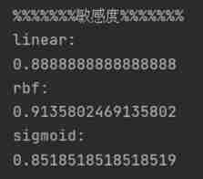
print("%%%%%%% Accuracy %%%%%%%")
print("%%%%%%% Sensitivity %%%%%%%")
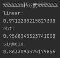
print("%%%%%%% Special effects %%%%%%%")
print("%%%%%%%F1_score%%%%%%%")
kernelList = ['linear','rbf','sigmoid']
for kernel in kernelList:
svc = SVC(kernel=kernel).fit(train_X,train_y)
y_pred = svc.predict(test_X)
# Calculation accuracy
score_svc = metrics.accuracy_score(test_y,y_pred)
print(kernel+":")
print(score_svc)
# Calculate recall rate ( Sensitivity )
print(recall_score(test_y, y_pred))
# Confusion matrix
C = confusion_matrix(test_y, y_pred)
TN=C[0][0]
FP=C[0][1]
FN=C[1][0]
TP=C[1][1]
# Calculate specific effect
specificity=TN/(TN+FP)
print(specificity)
# Calculation f1_score
# print(f1_score(test_y, y_pred))
# print(classification_report(test_y, y_pred))
7、 ... and 、 Run a screenshot
The following are the accuracy of the three kernel function models , Sensitivity , Special effect result :
   | |
For a more intuitive view of SVM Three kernel functions establish the performance measurement of the model , Draw the results into a table as follows ( Keep five decimal places ):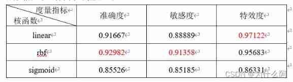
It can be seen from the table that , For this dataset , Kernel function rbf The accuracy and sensitivity of the established model are higher than the other two kernel functions , The special effect is slightly lower than linear Kernel function model , On the whole , Kernel function rbf The established classification model has better performance when applied to this dataset .
8、 ... and 、 Complete code
import matplotlib
import pandas as pd
import matplotlib.pyplot as plt
import seaborn as sns
from sklearn.metrics import classification_report, confusion_matrix
from sklearn.model_selection import train_test_split
from sklearn import svm
from sklearn.preprocessing import StandardScaler
from sklearn.svm import SVC
from sklearn import metrics
from sklearn.metrics import recall_score
from sklearn.metrics import f1_score
#  Solve the confusion of negative sign of coordinate axis scale
plt.rcParams['axes.unicode_minus'] = False
#  Solve the problem of Chinese garbled code
plt.rcParams['font.sans-serif'] = ['Simhei']
#  Show all columns of the dataset
pd.set_option('display.max_columns', None)

# Reading data sets
data = pd.read_excel(' Classification job data set .xlsx')
# Dataset view
print(data.info())
print(data.columns)
print(data.head(5))
print(data.describe())

# Data cleaning
#“ID" Columns have no practical significance , Delete
data.drop('ID',axis = 1,inplace=True)
# Will be of type B,M use 0,1 Instead of
data[' type '] = data[' type '].map({
    'M':1,'B':0})
#  The characteristic field is placed in features_mean
features_mean= list(data.columns[1:12])
#  Visualize two types of distribution
sns.countplot(x=" type ",data=data)
plt.show()
#  Present... With a heat map features_mean Correlation between fields
corr = data[features_mean].corr()
plt.figure(figsize=(14,14))
# annot=True Display data for each grid
sns.heatmap(corr, annot=True)
plt.show()
#  After feature selection 6 Features
features_remain = ['radius','texture', 'smoothnesscompactness','compactness','symmetry ', 'fractal dimension ']

# extract 40% As a test set , rest 60% As a training set
train,test = train_test_split(data,test_size = 0.4)
train_X = train[features_remain]   # Extract the value of feature selection as training and test data
train_y = train[' type ']
test_X = test[features_remain]
test_y = test[' type ']

# use Z-Score Standardization , Ensure that the data mean of each feature dimension is 0, The variance of 1
ss = StandardScaler()
train_X = ss.fit_transform(train_X)
test_X = ss.transform(test_X)

print("%%%%%%% Accuracy %%%%%%%")
print("%%%%%%% Sensitivity %%%%%%%")
print("%%%%%%% Special effects %%%%%%%")
print("%%%%%%%F1_score%%%%%%%")
kernelList = ['linear','rbf','sigmoid']
for kernel in kernelList:
    svc = SVC(kernel=kernel).fit(train_X,train_y)
    y_pred = svc.predict(test_X)
    #  Calculation accuracy
    score_svc = metrics.accuracy_score(test_y,y_pred)
    print(kernel+":")
    print(score_svc)
    #  Calculate recall rate ( Sensitivity )
    print(recall_score(test_y, y_pred))
    #  Confusion matrix
    C = confusion_matrix(test_y, y_pred)
    TN=C[0][0]
    FP=C[0][1]
    FN=C[1][0]
    TP=C[1][1]
    #  Calculate specific effect
    specificity=TN/(TN+FP)
    print(specificity)

    #  Calculation f1_score
    # print(f1_score(test_y, y_pred))
    # print(classification_report(test_y, y_pred))
边栏推荐
- ECMAScript--》 ES6语法规范 ## Day1
- One click generate traffic password (exaggerated advertisement title)
- Synchronous vs asynchronous
- Octave instructions
- Vgg16 migration learning source code
- Cases of OpenCV image enhancement
- Pycharm cannot import custom package
- Leetcode-513: find the lower left corner value of the tree
- 3.1 Monte Carlo Methods & case study: Blackjack of on-Policy Evaluation
- Implementation of "quick start electronic" window dragging
猜你喜欢

2.1 Dynamic programming and case study: Jack‘s car rental
Rewrite Boston house price forecast task (using paddlepaddlepaddle)

openCV+dlib實現給蒙娜麗莎換臉
3.1 Monte Carlo Methods & case study: Blackjack of on-Policy Evaluation
Leetcode-112:路径总和

LeetCode - 705 设计哈希集合(设计)

LeetCode - 1670 设计前中后队列(设计 - 两个双端队列)

Leetcode interview question 17.20 Continuous median (large top pile + small top pile)
![[LZY learning notes -dive into deep learning] math preparation 2.1-2.4](/img/92/955df4a810adff69a1c07208cb624e.jpg)
[LZY learning notes -dive into deep learning] math preparation 2.1-2.4
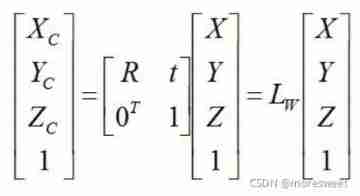
CV learning notes - camera model (Euclidean transformation and affine transformation)
随机推荐
Dynamic layout management
LeetCode - 673. Number of longest increasing subsequences
20220531数学:快乐数
[LZY learning notes dive into deep learning] 3.5 image classification dataset fashion MNIST
1. Finite Markov Decision Process
One click generate traffic password (exaggerated advertisement title)
Rewrite Boston house price forecast task (using paddlepaddlepaddle)
Opencv feature extraction - hog
Inverse code of string (Jilin University postgraduate entrance examination question)
[C question set] of Ⅵ
20220608 other: evaluation of inverse Polish expression
重写波士顿房价预测任务(使用飞桨paddlepaddle)
Opencv image rotation
Leetcode - 5 longest palindrome substring
波士顿房价预测(TensorFlow2.9实践)
20220604 Mathematics: square root of X
About windows and layout
Pytorch ADDA code learning notes
Opencv feature extraction sift
20220609 other: most elements