当前位置:网站首页>[LZY learning notes dive into deep learning] 3.1-3.3 principle and implementation of linear regression
[LZY learning notes dive into deep learning] 3.1-3.3 principle and implementation of linear regression
2022-07-03 10:18:00 【DadongDer】
The third chapter Linear neural networks
Introduce nerves ⽹ The whole training process of Luo , Include : Define simple nerves ⽹ Network structure 、 Data processing 、 Specify the loss function and how to train the model .
3.1 Linear regression
Return to regression It is a kind of method that can model the relationship between one or more independent variables and dependent variables . Regression is often used to represent the relationship between input and output , Related to prediction tasks
3.1.1 Linear regression linear regression The basic elements of
Linear regression is the standard of regression ⼯ It's the simplest and the most flow ⾏.
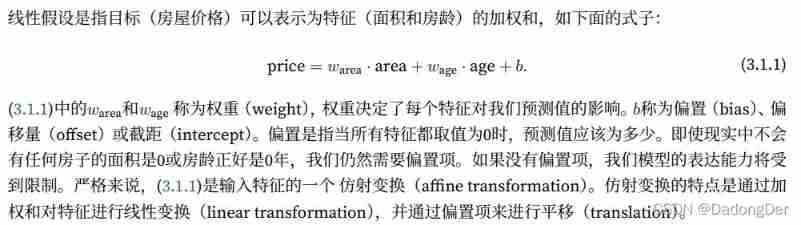
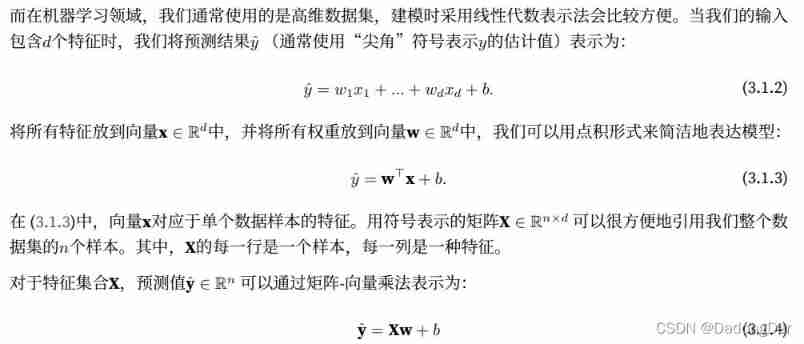
Linear regression is based on simple assumptions :⾸ First , hypothesis ⾃ Variable x And dependent variables y The relationship is linear , namely y You can watch ⽰ by x Of the elements of Weighted sums , this ⾥ It is usually allowed to include observations ⼀ Some noise ; secondly , Let's assume that any noise ⽐ More normal , If the noise follows a normal distribution .
Proper noun :
For development ⼀ A model that can predict house prices , We need to collect ⼀ A real data set . This data set includes the sales price of the house 、⾯ Accumulation and housing age . In the terminology of machine learning , This data set is called the training data set (training data set) Or training set (training set).
Every time ⾏ data (⽐ Such as ⼀ Data corresponding to this housing transaction ) Called a sample (sample), It can also be called data point (data
point) Or data samples (data instance).
We try to predict ⽬ mark (⽐ Such as predicting house prices ) It's called a tag (label) or ⽬ mark (target).
The prediction is based on ⾃ Variable (⾯ Accumulation and housing age ) be called features (feature) Or covariates (covariate).
Linear model

Start looking for the best model parameters (model parameters)w and b Before , We need two more things :(1)⼀ A measure of model quality ⽅ type ;(2)⼀ A method that can update the model to improve ⾼ Model prediction quality ⽅ Law .
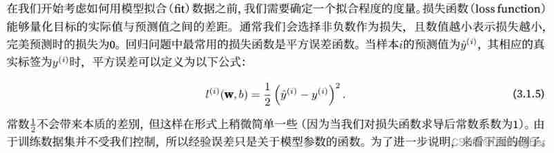
Loss function

Analytic solution

Stochastic gradient descent
Even in us ⽆ When the analytical solution is obtained by the method , We can still train the model effectively . Figure out how to train these models that are difficult to optimize .
gradient descent (gradient descent) such ⽅ Law ⼏ Almost all deep learning models can be optimized . It is achieved by continuously decreasing the loss function ⽅ Update the parameters up to reduce the error .
Gradient descent is the simplest ⽤ The method is to calculate the loss function ( The mean loss of all samples in the data set ) About the derivative of model parameters ( Here ⾥ It can also be called gradient ). But in practice ⾏ May be ⾮ Often slow : Because in every ⼀ Before the parameters are updated again , We have to traverse the entire data set . therefore , We usually take random samples every time we need to calculate the update ⼀ A small batch of samples , This variant is called Small batch random gradient drop (minibatch stochastic gradient descent).

Using models to make predictions 
3.1.2 Vectorization acceleration
When training our model , We often It is hoped that the whole small batch of samples can be processed at the same time . In order to do that ⼀ spot , We need to calculate ⾏⽮ quantitative , Thus benefit ⽤ Linear algebra library , Not in Python Writing overhead ⾼ High for loop .
import math
import time
import numpy as np
import torch

#  Into the ⾏ Benchmark of running time , Definition ⼀ Timers
class Timer:
    def __init__(self): #  Record multiple run times
        self.times = []
        self.tik = None
        self.start()

    def start(self): #  Start the timer
        self.tik = time.time()

    def stop(self): #  Stop the timer and record the time in the list
        self.times.append(time.time() - self.tik)
        return self.times[-1] #  Go back to the last

    def avg(self): #  Return to average time
        return sum(self.times) / len(self.times)

    def sum(self): #  Returns the total time
        return sum(self.times)

    def cumsum(self): #  Returns the cumulative time
        return np.array(self.times).cumsum().tolist()

#  Benchmark the workload
#  Test the load of the two methods of vector addition
n = 10000
a = torch.ones(n)
b = torch.ones(n)
c = torch.zeros(n)
timer = Timer()
for i in range(n):
    c[i] = a[i] + b[i]
print(f'{
      timer.stop(): .5f} sec')

timer.start()
d = a + b
print(f'{
      timer.stop(): .5f} sec')
⽮ Quantifying code usually brings about an order of magnitude of acceleration
Put more mathematical operations into the Library , and ⽆ Must be ⾃⼰ Write so many calculations , This reduces the possibility of error
3.1.3 Normal distribution and square loss
Normal distribution 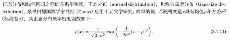
Changing the average will produce ⽣ Along the x The offset of the axis , increase ⽅ The difference will be dispersed 、 Reduce its peak value .
import math
import numpy as np
import matplotlib.pyplot as plt

#  Calculate the normal distribution
def normal(x, mu, sigma):
    p = 1 / math.sqrt(2 * math.pi * sigma ** 2)
    return p * np.exp(-0.5 / sigma ** 2 * (x - mu) ** 2)

#  Visualizing normal distribution
x = np.arange(-7, 7, 0.01)
params = [(0, 1), (0, 2), (3, 1)] #  Mean and standard deviation pair
for mu, sigma in params:
    plt.plot(x, normal(x, mu, sigma), label=f'mean {
      mu}, std {
      sigma}')

plt.xlabel("x")
plt.ylabel("p(x)")
plt.legend()
plt.show()
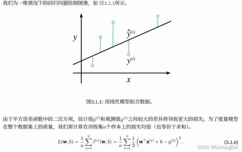
Mean square error loss function ( Mean square loss )
Explain why the mean square error can be used in linear regression :
Suppose the observation contains noise , The noise obeys normal distribution
Under the assumption of Gaussian noise , Minimizing the mean square error is equivalent to the maximum likelihood estimation of the linear model 
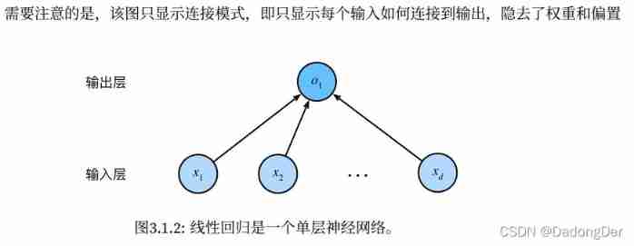
3.1.4 From linear regression to depth network
Neural network diagram

biology
Today, ⼤ Most studies of deep learning ⼏ Almost no direct inspiration from neuroscience . Nowadays, inspiration in deep learning comes equally or more ⾃ mathematics 、 Statistics and computer science .
Summary
• The key element in machine learning model is training data 、 Loss function 、 optimization algorithm , And the model book ⾝.
• ⽮ Quantification makes mathematical expression more concise , Simultaneous transportation ⾏ Faster .
• To minimize the ⽬ Scalar function and execution ⾏ extremely ⼤ Likelihood estimation is equivalent .
• The linear regression model is also ⼀ A simple nerve ⽹ Collateral .
3.2 Linear regression is realized from zero
3.2.1 Generate data set
⽣ become ⼀ Contains 1000 The data set of 2 samples , Each sample contains samples from the standard normal distribution 2 Features .
The composite dataset is ⼀ Matrix X ∈ R1000×2.
detach() detach_() data difference
3.2.2 Reading data sets
When training the model, the data set should be ⾏ Traverse , Every time I draw ⼀ Small batch samples , And make ⽤ They update our model . Because this process is the basis of training machine learning algorithms , So it is necessary to define ⼀ A function , This function can scramble the samples in the data set and ⽅ Get data in the form of .
random.shuffle
python for range loop
python yield
3.2.3 Initialize model parameters
After initializing parameters , Our task is to update these parameters , Until these parameters ⾜ Enough to fit our data . Each update needs to calculate the gradient of the loss function with respect to the model parameters . With this gradient , We can reduce the loss to ⽅ Update each parameter to .
because ⼿ Dynamic gradient calculation is boring and error prone , So there was no ⼈ Meeting ⼿ Dynamically calculate the gradient . We make ⽤ 2.5 Mid section quotation ⼊ Of ⾃ Dynamic differential to calculate the gradient .
3.2.4 Defining models
Defining models , Input the model ⼊ And parameters are associated with the output of the model
3.2.5 Define the loss function
3.2.6 optimization algorithm : Small batch random gradient descent method
In each of the ⼀ In step , send ⽤ Randomly selected from a data set ⼀ A small batch , Then the gradient of loss is calculated according to the parameters . Next , Towards reducing losses ⽅ Update our parameters to .
torch.no_grad()
3.2.7 Training process
The training process has something in common . Deep learning is almost the same training process
.backward
.sum The gradient of 1 It doesn't affect the result Only scalars can backward
In each iteration , Read a small batch of training samples , And get a set of predictions through the model . After calculating the loss , Start backpropagation , Store the gradient of each parameter . Finally, call the optimization algorithm to update the model parameters .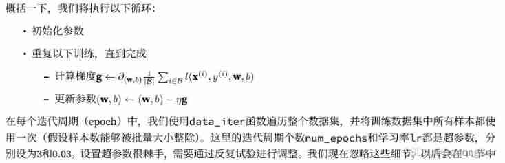
We should not take it for granted that we can solve the parameters perfectly . In machine learning , We usually don't care much ⼼ Restore the real parameters , And more close ⼼ how ⾼ Accuracy prediction parameters . Fortunately, , Even in complex optimization problems , Random gradient descent can also be found ⾮ A good solution . among ⼀ One reason is , At depth ⽹ There are many parameter combinations in the network that can realize ⾼ Accurate prediction .
import random
import torch
import matplotlib.pyplot as plt

# 3.2.1  Generate data set

# ease to understand
# X = torch.normal(0, 1, (5, 2)) #  Normal distribution   mean value , Standard deviation ,size
# print(X)
# w = torch.tensor([2, -3.4])
# print(w)
# y = torch.matmul(X, w) # matrix multiple  Matrix multiplication
# print(y)
# print(y.shape)
# print(y.reshape(-1, 1)) # -1  Auto fill   The given column determines here


#  Generate data set  y=Xw+b+ noise
def synthetic_data(w, b, num_examples):
    #  Yes X:  Yes num_examples Samples   Each sample has len(w) Features
    X = torch.normal(0, 1, (num_examples, len(w))) # len(w)  Because  matmul(X, w)
    y = torch.matmul(X, w) + b
    #  Random noise   Set here to obey the mean value 0 Is a normal distribution , The standard deviation is set to 0.01
    y += torch.normal(0, 0.01, y.shape) # +=  No new memory will be allocated
    return X, y.reshape((-1, 1))

# step 1  Generation contains 1000 The data set of 2 samples , Each sample contains samples from the standard normal distribution 2 Features
true_w = torch.tensor([2, -3.4]) # 2 Weighted sum of features , So we need to [w1,w2]
true_b = 4.2
features, labels = synthetic_data(true_w, true_b, 1000)

#  See function synthetic_data  among features: num_examples * len(w) label: -1 * 1
print('features:', features[0], '\nlabel:', labels[0]) #  Output [0] first line

# step 2  visualization
#  Draw the second 2 Eigenvalues   and  labels  The scatter diagram of  y=w1x1+w2x2+b+ noise   It should be linear
# detach() Create the same data as the original , Share data with the original , The two changes are consistent , however detach() The latter cannot be derived and the derivation will report an error
# numpy() Convert to array
plt.scatter(features[:, 1].detach().numpy(), labels.detach().numpy(), 1)    # point_size = 1
plt.show()


# 3.2.2  Reading data sets
#  When training the model, the data set should be ⾏ Traverse , Every time I draw ⼀ Small batch samples , And use them to update our model .

#  This function receives the batch size 、 Feature matrix and label vector are used as input
#  The generation size is batch_size A small batch of , Each small batch contains ⼀ Group features and labels
def data_iter(batch_size, features, labels):
    num_examples = len(features)
    # list(range(5)) = list(range(0,5)) = [0,1,2,3,4]
    indices = list(range(num_examples))
    #  Sort all the elements of the sequence at random
    random.shuffle(indices)
    for i in range(0, num_examples, batch_size): # start end+1 step
        batch_indices = torch.tensor(indices[i: min(i + batch_size, num_examples)])
        yield features[batch_indices], labels[batch_indices]
    #  Iteration execution efficiency is low , May encounter trouble in practical problems

batch_size = 10
for X, y in data_iter(batch_size, features, labels):
    print(X, '\n', y)
    break #  Only one set of data is returned here   No break It will show all the divisions

# 3.2.3  Initialize model parameters

#  From the mean to 0、 The standard deviation is 0.01 Random numbers are sampled in the normal distribution to initialize the weight , And initialize the offset to 0
w = torch.normal(0, 0.01, size=(2, 1), requires_grad=True)
# print(f'w: {w}')
b = torch.zeros(1, requires_grad=True)

# 3.2.4  Defining models

def linreg(X, w, b):
    return torch.matmul(X, w) + b
    # b Scalar   Matrix multiplication vector   Adding is the broadcasting mechanism
    # ⽤⼀ Vector plus ⼀ Scalar , Scalars are added to each component of the vector .

# 3.2.5  Define the loss function

def squared_loss(y_hat, y):
    return (y_hat - y.reshape(y_hat.shape)) ** 2 / 2 #  Square loss function

# 3.2.6  Define optimization algorithms : Small batch random gradient drop

def sgd(params, lr, batch_size): #  Model parameter set 、 Learning rate and batch size as input ⼊
    #  Every time ⼀ Step updated ⼤ Xiaoyou learning rate lr decision
    with torch.no_grad(): #  Do not build the calculation diagram
        for param in params:
            param -= lr * param.grad / batch_size #  Update our parameters in the direction of reducing losses
            param.grad.zero_()

# 3.2.7  Training

lr = 0.03 #  Set the super parameter learning rate
num_epochs = 5 #  Set the super parameter period
net = linreg
loss = squared_loss

for epoch in range(num_epochs):
    for X, y in data_iter(batch_size, features, labels): #  Keep updating iteratively w b
        l = loss(net(X, w, b), y)
        l.sum().backward() # .sum Scalar
        sgd([w, b], lr, batch_size) #  Derivative update w b
    with torch.no_grad():
        train_l = loss(net(features, w, b), labels)
        print(f'epoch {
      epoch + 1}, loss {
      float(train_l.mean()): f}')

print(f'error in estimating w: {
      true_w - w.reshape(true_w.shape)}')
print(f'error in estimating b: {
      true_b - b}')
Summary
• We learned depth ⽹ How to realize and optimize the network . Here ⼀ In the process, only ⽤ Tensors and automatic differentiation , There is no need to define layers or complex optimizers .
• this ⼀ Section only touches the table ⾯ knowledge . In the following section , We will describe other models based on the concepts just introduced , And learn how to implement other models more succinctly .
3.3 Simple realization of linear regression ( rely on API)
import numpy as np
import torch
from torch.utils import data
from torch import nn

# step 1  Generate data set
def synthetic_data(w, b, num_examples):
    X = torch.normal(0, 1, (num_examples, len(w)))
    y = torch.matmul(X, w) + b
    y += torch.normal(0, 0.01, y.shape)
    return X, y.reshape((-1, 1))

true_w = torch.tensor([2, -3.4])
true_b = 4.2
features, labels = synthetic_data(true_w, true_b, 100)

# step 2  Reading data sets
def load_array(data_arrays, batch_size, is_train=True): #  Construct data iterators
    dataset = data.TensorDataset(*data_arrays)
    return data.DataLoader(dataset, batch_size, shuffle=is_train)
    # shuffle set to ``True`` to have the data reshuffled at every epoch

batch_size = 10
data_iter = load_array((features, labels), batch_size)
# print(next(iter(data_iter))) # https://www.runoob.com/python3/python3-iterator-generator.html

# step 3  Defining models
# note 1:  Definition ⼀ Model variables net, It is ⼀ individual Sequential Class .Sequential Class standard assembly line
# Sequential Class concatenates multiple layers in ⼀ rise . When a given input ⼊ Data time ,Sequential Instance transmits data ⼊ To the first ⼀ layer , And then I will ⼀ The output of the layer is the first ⼆ Layer transport ⼊, And so on .
# note 2:  Single layer network architecture , this ⼀ A single layer is called a fully connected layer (fully-connected layer)
#  Because of its every ⼀ A loss ⼊ Through the matrix - Vector multiplication yields each of its outputs .
#  stay PyTorch in , The full connection layer is in Linear Definition in class . Two parameters ( Specify input ⼊ Feature shape , Specify the output shape )
net = nn.Sequential(nn.Linear(2, 1))

# step 4  Initialize model parameters
net[0].weight.data.normal_(0, 0.01) #  The first layer of the network / Access data / Set parameters
net[0].bias.data.fill_(0)

# step 5  Define the loss function
loss = nn.MSELoss() #  By default , It returns the average of all sample losses

# step 6  Define optimization algorithms
#  Specify optimized parameters ( It can be done by net.parameters() From our model ) And the super parameter dictionary required by the optimization algorithm
trainer = torch.optim.SGD(net.parameters(), lr=0.03)

# step 7  Training
num_epochs = 5
for epoch in range(num_epochs):
    for X, y in data_iter:
        l = loss(net(X), y)
        trainer.zero_grad()
        l.backward()
        trainer.step() # Performs a single optimization step (parameter update).
    l = loss(net(features), labels)
    print(f'epoch {
      epoch + 1}, loss {
      l: f}')

w = net[0].weight.data
b = net[0].bias.data
print(f'error in estimating w: {
      true_w - w.reshape(true_w.shape)}')
print(f'error in estimating b: {
      true_b - b}')
Summary
• We can make ⽤PyTorch Of ⾼ level API Implement the model more concisely .
• stay PyTorch in ,data The module provides data processing ⼯ have ,nn Module defines ⼤ Amount of nerve ⽹ Complex layer and Chang ⻅ Loss function .
• We can go through _ At the end of the ⽅ Method to replace the parameter , This initializes the parameters .
边栏推荐
- LeetCode - 933 最近的请求次数
- Deep Reinforcement learning with PyTorch
- . DLL and Differences between lib files
- The data read by pandas is saved to the MySQL database
- 20220610 other: Task Scheduler
- Yocto technology sharing phase IV: customize and add software package support
- Connect Alibaba cloud servers in the form of key pairs
- Adaptiveavgpool1d internal implementation
- Leetcode - 1670 conception de la file d'attente avant, moyenne et arrière (conception - deux files d'attente à double extrémité)
- Leetcode - 1670 design front, middle and rear queues (Design - two double ended queues)
猜你喜欢
LeetCode - 1670 设计前中后队列(设计 - 两个双端队列)

Deep learning by Pytorch
Leetcode interview question 17.20 Continuous median (large top pile + small top pile)
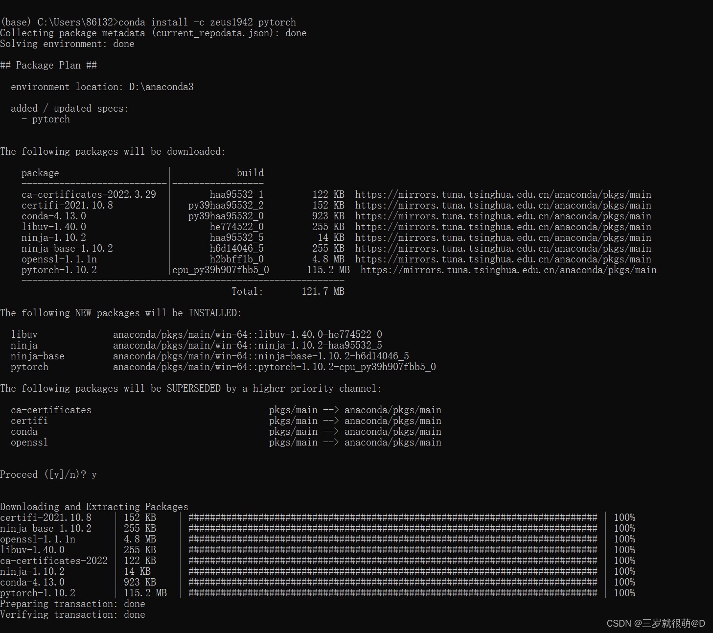
Anaconda安装包 报错packagesNotFoundError: The following packages are not available from current channels:

Label Semantic Aware Pre-training for Few-shot Text Classification
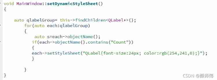
QT is a method of batch modifying the style of a certain type of control after naming the control

Leetcode 300 最长上升子序列

LeetCode - 705 设计哈希集合(设计)
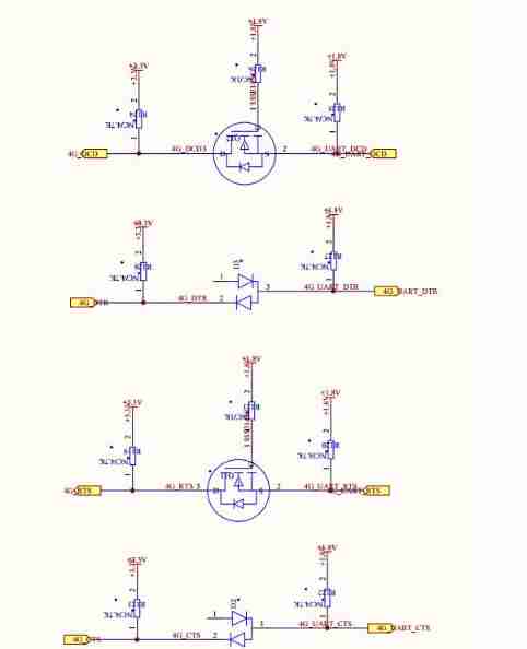
My notes on intelligent charging pile development (II): overview of system hardware circuit design

Connect Alibaba cloud servers in the form of key pairs
随机推荐
Vgg16 migration learning source code
My 4G smart charging pile gateway design and development related articles
Leetcode 300 最长上升子序列
重写波士顿房价预测任务(使用飞桨paddlepaddle)
Swing transformer details-1
20220610其他:任务调度器
Retinaface: single stage dense face localization in the wild
2312、卖木头块 | 面试官与狂徒张三的那些事(leetcode,附思维导图 + 全部解法)
Label Semantic Aware Pre-training for Few-shot Text Classification
Window maximum and minimum settings
Opencv note 21 frequency domain filtering
2.1 Dynamic programming and case study: Jack‘s car rental
Dictionary tree prefix tree trie
LeetCode - 900. RLE 迭代器
CV learning notes convolutional neural network
Leetcode - 895 maximum frequency stack (Design - hash table + priority queue hash table + stack)*
20220604数学:x的平方根
CV learning notes - edge extraction
2312. Selling wood blocks | things about the interviewer and crazy Zhang San (leetcode, with mind map + all solutions)
【毕业季】图匮于丰,防俭于逸;治不忘乱,安不忘危。