[LZY learning notes dive into deep learning] 3.4 3.6 3.7 softmax principle and Implementation

d2l The meaning of existence is to save all the previously declared functions , Pass for the first time @save The mark is automatically recorded , You can call it directly in the future .d2l Completely replaceable .

3.4 softmax Return to

Return to vs classification

Return to ：“ How many? ”
classification ：“ Which one ”
A situation , Only care about hard categories （ Which category does the sample belong to ）, But still use the soft category model （ The probability of belonging to each category ）

3.4.1 Classification problem

Method of representing classified data ： Hot coding alone one-hot encoding
The unique heat code is a vector , There are as many components as categories ;
The component corresponding to the category is set to 1, All other components are set to 0.
for example ：y∈{(1,0,0),(0,1,0),(0,0,1)}

3.4.2 Network architecture

In order to estimate the conditional probabilities of all possible categories , Need a model with multiple outputs , Each category corresponds to an output .
In order to solve the classification problem of linear model , Need and output ⼀ How many affine functions （affine function）.
Each output corresponds to its own affine function .

The vector form is expressed as o = Wx + b

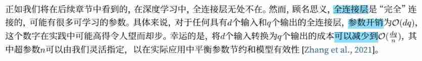
3.4.3 The parameter overhead of the whole connection layer

3.4.4 softmax operation

need ：
① I hope the output of the model yˆj Can be regarded as belonging to class j Probability , Then select the category with the largest output value argmaxj yj As our prediction
②** You can't put an unregulated forecast o Directly see the output of interest .** Because the output of the linear layer is directly
When regarded as probability, there is ⼀ Some questions ： There is no limit to the sum of these output numbers 1; Different input , It can be negative . These violate the basic axioms of probability .
③ need ⼀ Training objectives to encourage the model to accurately estimate the probability . In the classifier output 0.5 Of all samples , I hope these samples have ⼀ Semi actually belongs to the class of prediction . This property is called calibration （calibration）
Qualified models are generated ：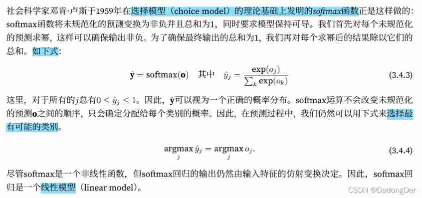

3.4.5 Vectorization of small batch samples

3.4.6 Loss function ： Maximum likelihood estimation

Log likelihood

softmax And its derivative

Cross entropy loss
send ⽤ (3.4.8) To define loss l, It is the expected loss value of all label distributions . This loss is called cross entropy loss （crossentropy loss）, It is the most common classification problem ⽤ Loss of ⼀.

3.4.7 The basis of information theory

entropy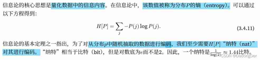

Amazed
The relationship between compression and prediction ： When data is easy to predict , It's easy to compress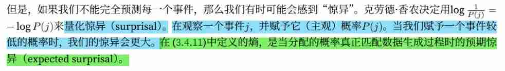

Cross entropy

3.4.8 Model prediction and evaluation

In the training softmax After the regression model , Give any sample characteristics , We can predict the probability of each output category . Usually we make ⽤ The prediction probability is the most ⾼ As the output category . If forecast and actual category （ label ）⼀ Cause , Then the prediction is correct .
In the next experiment , We will make ⽤ precision （accuracy） To evaluate the performance of the model . The accuracy is equal to the difference between the correct prediction number and the total prediction number ⽐ rate .
Summary
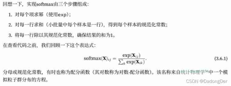
• softmax Computing to get ⼀ Vector and map it to probability .
• softmax Return to fitness ⽤ This paper focuses on the problem of classification , It makes ⽤ 了 softmax The probability distribution of the output category in the operation .
• The cross entropy is zero ⼀ A good measure of the difference between two probability distributions , It measures what is needed to encode data for a given model ⽐ Special number .

3.6 softmax Return from scratch

Cross entropy loss function

import torch
import commfuncs
import time
import torch
import torchvision
from torch.utils import data
from torchvision import transforms
import matplotlib.pyplot as plt

def get_dataloader_workers():
    return 0

def load_data_fashion_mnist(batch_size, resize=None):
    trans = [transforms.ToTensor()]
    if resize:
        trans.insert(0, transforms.Resize(resize))
    trans = transforms.Compose(trans)
    # print(trans)

    mnist_train = torchvision.datasets.FashionMNIST(root="../data", train=True, transform=trans, download=True)
    mnist_test = torchvision.datasets.FashionMNIST(root="../data", train=False, transform=trans, download=True)

    return (data.DataLoader(mnist_train, batch_size, shuffle=True, num_workers=get_dataloader_workers()),
            data.DataLoader(mnist_test, batch_size, shuffle=False, num_workers=get_dataloader_workers()))

# 0:  Loading data sets 
batch_size = 256
train_iter, test_iter = load_data_fashion_mnist(batch_size)

# 1:  Initialize model parameters 
num_inputs = 784 # 28*28  Flatten the image into a vector   Each pixel position is regarded as a feature 
num_outputs = 10 #  The dataset has 10 Categories 

#  Each output corresponds to an affine function 
# o1 = w11 x1 + w12 x2 + ... + w1784 x784 + b1
# 02 = w21 x1 + w22 x2 + ... + w2784 x784 + b2
# ...
# o10 = w101 x1 + w102 x2 + ... + w10784 x784 + b10
# W: 10 * 784 b: 10 * 1 -> W: 784*10 b:1*10

W = torch.normal(0, 0.01, size=(num_inputs, num_outputs), requires_grad=True)
b = torch.zeros(num_outputs, requires_grad=True)
# print(W.shape)

# X = torch.tensor([[1.0, 2.0, 3.0], [4.0, 5.0, 6.0]])
# print(X.sum(0, keepdim=True)) #  Keep going   By column 
# tensor([[5., 7., 9.]])
# print(X.sum(1, keepdim=True)) #  Keep the column   By line 
# tensor([[ 6.],
# [15.]])


# 2:  Definition softmax operation   Conform to the probability theorem 
def softmax(X):
    X_exp = torch.exp(X)
    # print(X_exp)
    partition = X_exp.sum(1, keepdim=True) #  Keep the column   By line 
    # print(partition)
    return X_exp / partition

# X = torch.normal(0, 1, (2, 5))
# print(X)
# X_prob = softmax(X)
# print(X_prob)
# print(X_prob.sum(1))

# 3:  Defining models 
#  transport ⼊ How to map to the output through the network 
# reshape Function flattens each original image into a vector 
# O = XW + b
# ^Y = softmax(O)
def net(X):
    return softmax(torch.matmul(X.reshape((-1, W.shape[0])), W) + b)

# 4:  Define the loss function 
y = torch.tensor([0, 2])
y_hat = torch.tensor([[0.1, 0.3, 0.6], [0.3, 0.3, 0.5]])
# print(y_hat[[0, 1], y])
# x y  Correspond in sequence  array[[x1,x2,x3],[y1,y2,y3]] ->(x1,y1)(x2,y2)(x3,y3)

def cross_entropy(y_hat, y):
    # print(len(y_hat))
    # print(range(len(y_hat)))
    # print(y_hat[range(len(y_hat)), y])
    return - torch.log(y_hat[range(len(y_hat)), y]) # https://zhuanlan.zhihu.com/p/35709485
# print(cross_entropy(y_hat, y)) #  Ask in sequence log

# 5:  Classification accuracy 
def accuracy(y_hat, y): #y_hat  Prediction probability distribution 
    # print(y_hat, y_hat.shape, y_hat.dtype)
    if len(y_hat.shape) > 1 and y_hat.shape[1] > 1:
        # y_hat It's a matrix   Suppose that the second dimension stores the predicted score of each class 
        # argmax Get the index of the largest element in each row to get the prediction category 
        y_hat = y_hat.argmax(axis=1)
        # print(y_hat, y_hat.shape, y_hat.dtype)
    cmp = y_hat.type(y.dtype) == y #  The result is to include 0 1  Tensor 
    return float(cmp.type(y.dtype).sum())

# print(accuracy(y_hat, y) / len(y))

# tensor([[0.1000, 0.3000, 0.6000],
# [0.3000, 0.3000, 0.5000]]) torch.Size([2, 3]) torch.float32
# tensor([2, 2]) torch.Size([2]) torch.int64
# 0.5

#  For any data iterator data_iter Accessible data sets , Can be evaluated in any model net The accuracy of the 
#  Calculates the accuracy of the model on the specified data set 
def evaluate_accuracy(net, data_iter):
    if isinstance(net, torch.nn.Module):      # in this example, False
        net.eval()
    metric = Accumulator(2) #  Correct prediction number   The total number of predictions ;  When traversing the dataset, both will accumulate over time 
    with torch.no_grad():
        for X, y in data_iter:
            metric.add(accuracy(net(X), y), y.numel())
    return metric[0] / metric[1]

#  Accumulate multiple variables 
class Accumulator:
    def __init__(self, n):
        self.data = [0.0] * n

    def add(self, *args):
        self.data = [a + float(b) for a, b in zip(self.data, args)]

    def reset(self):
        self.data = [0.0] * len(self.data)

    def __getitem__(self, idx):
        return self.data[idx]

# print(evaluate_accuracy(net, test_iter)) # the accuracy is approximately 1/10 as the network has not been trained

#  The training model has an iterative cycle 
def train_epoch_ch3(net, train_iter, loss, updater):
    #  Set the model to training mode 
    if isinstance(net, torch.nn.Module):      # in this example, False
        net.train()
    #  The sum of training losses 、 Total training accuracy 、 Sample size 
    metric = Accumulator(3)
    for X, y in train_iter:
        #  Calculate the gradient and update the parameters 
        y_hat = net(X)
        l = loss(y_hat, y)
        if isinstance(updater, torch.optim.Optimizer):      # in this example, False
            #  Use pytorch Built in optimizer and loss function 
            updater.zero_grad()
            l.mean().backward()
            updater.step()
        else:
            #  Use custom optimizers and loss functions 
            l.sum().backward()
            updater(X.shape[0])
        metric.add(float(l.sum()), accuracy(y_hat, y), y.numel())
    #  Return training loss and training accuracy 
    return metric[0] / metric[2], metric[1] / metric[2]

def sgd(params, lr, batch_size):
    with torch.no_grad():
        for param in params:
            param -= lr * param.grad / batch_size
            param.grad.zero_()

def train_ch3(net, train_iter, test_iter, loss, num_epochs, updater):
    for epoch in range(num_epochs):
        train_metrics = train_epoch_ch3(net, train_iter, loss, updater)
        train_loss, train_acc = train_metrics
        test_acc = evaluate_accuracy(net, test_iter)
        print(f'epoch {
      epoch + 1}, train_loss {
      float(train_loss): f}, train_acc {
      float(train_acc): f}, '
              f'test_acc {
      float(test_acc): f}')

lr = 0.1
#  Customized optimizer   Batch SGD
def updater(batch_size):
    return sgd([W, b], lr, batch_size)

num_epochs = 20
train_ch3(net, train_iter, test_iter, cross_entropy, num_epochs, updater)

def get_fashion_mnist_labels(labels):
    text_labels = ['t-shirt', 'trouser', 'pullover', 'dress', 'coat', 'sandal', 'shirt', 'sneaker', 'bag', 'ankle boot']
    return [text_labels[int(i)] for i in labels]

def show_images(imgs, num_rows, num_cols, titles=None):
    _, axes = plt.subplots(num_rows, num_cols)
    axes = axes.flatten()
    for i, (ax, img) in enumerate(zip(axes, imgs)):
        if torch.is_tensor(img):
            ax.imshow(img.numpy())
        else:
            ax.imshow(img)
        ax.axes.get_xaxis().set_visible(False)
        ax.axes.get_yaxis().set_visible(False)
        if titles:
            ax.set_title(titles[i])
    plt.show()

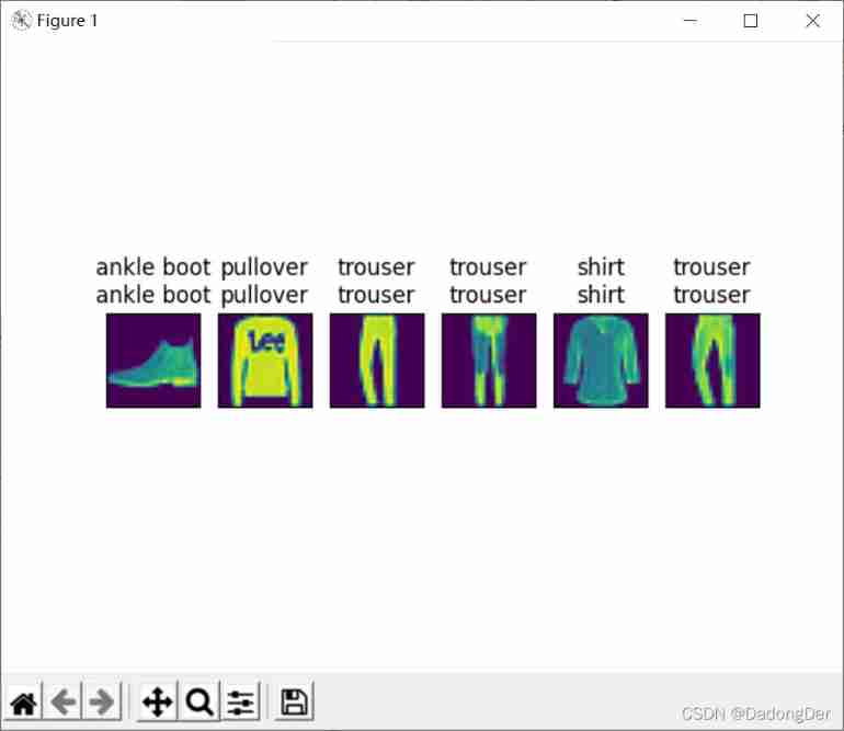
# step 7:  forecast 
def predict_ch3(net, test_iter, n=6):
    for X, y in test_iter:
        break
    trues = get_fashion_mnist_labels(y)
    preds = get_fashion_mnist_labels(net(X).argmax(axis=1))
    titles = [true + '\n' + pred for true, pred in zip(trues, preds)]
    show_images(X[0:n].reshape((n, 28, 28)), 1, n, titles=titles[0:n])

predict_ch3(net, test_iter)

Summary
• With the help of softmax Return to , We can train multi classification models .
• Training softmax Regression cycle model and training linear regression model ⾮ Often similar ： Read data first , Redefine the model and loss function , then
Use the optimization algorithm to train the model .⼤ Most often ⻅ Deep learning models have similar training processes .

3.7 softmax The simple realization of return

import torch
from torch import nn
from torchvision import transforms
import time
import torchvision
from torch.utils import data
from torchvision import transforms

def get_dataloader_workers():
    return 0

def load_data_fashion_mnist(batch_size, resize=None):
    trans = [transforms.ToTensor()]
    if resize:
        trans.insert(0, transforms.Resize(resize))
    trans = transforms.Compose(trans)
    # print(trans)

    mnist_train = torchvision.datasets.FashionMNIST(root="../data", train=True, transform=trans, download=True)
    mnist_test = torchvision.datasets.FashionMNIST(root="../data", train=False, transform=trans, download=True)

    return (data.DataLoader(mnist_train, batch_size, shuffle=True, num_workers=get_dataloader_workers()),
            data.DataLoader(mnist_test, batch_size, shuffle=False, num_workers=get_dataloader_workers()))

#  In average 0 And standard deviation 0.01 Random initialization weights 
def init_weights(m):
    if type(m) == nn.Linear:
        nn.init.normal_(m.weight, std=0.01)

class Accumulator:
    def __init__(self, n):
        self.data = [0.0] * n

    def add(self, *args):
        self.data = [a + float(b) for a, b in zip(self.data, args)]

    def reset(self):
        self.data = [0.0] * len(self.data)

    def __getitem__(self, idx):
        return self.data[idx]

def accuracy(y_hat, y): #y_hat  Prediction probability distribution 
    # print(y_hat, y_hat.shape, y_hat.dtype)
    if len(y_hat.shape) > 1 and y_hat.shape[1] > 1:
        # y_hat It's a matrix   Suppose that the second dimension stores the predicted score of each class 
        # argmax Get the index of the largest element in each row to get the prediction category 
        y_hat = y_hat.argmax(axis=1)
        # print(y_hat, y_hat.shape, y_hat.dtype)
    cmp = y_hat.type(y.dtype) == y #  The result is to include 0 1  Tensor 
    return float(cmp.type(y.dtype).sum())

#  For any data iterator data_iter Accessible data sets , Can be evaluated in any model net The accuracy of the 
#  Calculates the accuracy of the model on the specified data set 
def evaluate_accuracy(net, data_iter):
    if isinstance(net, torch.nn.Module):      # in this example, False
        net.eval()
    metric = Accumulator(2) #  Correct prediction number   The total number of predictions ;  When traversing the dataset, both will accumulate over time 
    with torch.no_grad():
        for X, y in data_iter:
            metric.add(accuracy(net(X), y), y.numel())
    return metric[0] / metric[1]

#  The training model has an iterative cycle 
def train_epoch_ch3(net, train_iter, loss, updater):
    #  Set the model to training mode 
    if isinstance(net, torch.nn.Module):      # in this example, False
        net.train()
    #  The sum of training losses 、 Total training accuracy 、 Sample size 
    metric = Accumulator(3)
    for X, y in train_iter:
        #  Calculate the gradient and update the parameters 
        y_hat = net(X)
        l = loss(y_hat, y)
        if isinstance(updater, torch.optim.Optimizer):      # in this example, False
            #  Use pytorch Built in optimizer and loss function 
            updater.zero_grad()
            l.mean().backward()
            updater.step()
        else:
            #  Use custom optimizers and loss functions 
            l.sum().backward()
            updater(X.shape[0])
        metric.add(float(l.sum()), accuracy(y_hat, y), y.numel())
    #  Return training loss and training accuracy 
    return metric[0] / metric[2], metric[1] / metric[2]

def sgd(params, lr, batch_size):
    with torch.no_grad():
        for param in params:
            param -= lr * param.grad / batch_size
            param.grad.zero_()

def train_ch3(net, train_iter, test_iter, loss, num_epochs, updater):
    for epoch in range(num_epochs):
        train_metrics = train_epoch_ch3(net, train_iter, loss, updater)
        train_loss, train_acc = train_metrics
        test_acc = evaluate_accuracy(net, test_iter)
        print(f'epoch {
      epoch + 1}, train_loss {
      float(train_loss): f}, train_acc {
      float(train_acc): f}, '
              f'test_acc {
      float(test_acc): f}')

batch_size = 256
train_iter, test_iter = load_data_fashion_mnist(batch_size)

# step 1  Initialize model parameters 
# PyTorch Does not implicitly adjust input ⼊ The shape of the . therefore ,
#  We defined the flattening layer before the linear layer （flatten）, To adjust ⽹ Collaterals ⼊ The shape of the 
net = nn.Sequential(nn.Flatten(), nn.Linear(784, 10))

net.apply(init_weights)
loss = nn.CrossEntropyLoss(reduction='none')
trainer = torch.optim.SGD(net.parameters(), lr=0.1)

num_epochs = 10
train_ch3(net, train_iter, test_iter, loss, num_epochs, trainer)

loss = nn.CrossEntropyLoss(reduction=‘none’)
Yes softmax Re examination and implementation of （ Solve numerical instability ： Overflow 、 underflow 、 Index calculation ）
Solution ： Cross entropy softmax Combination
Overflow ：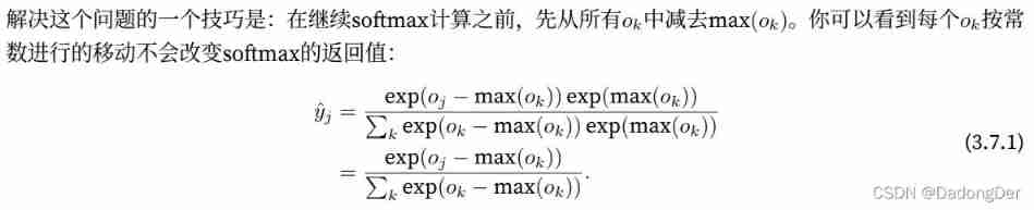

underflow 、 Index calculation ：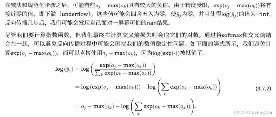

I hope to keep the traditional softmax function , In case we need to evaluate the probability of output through the model . however , We didn't softmax The probability is transferred to the loss function , Instead, the non normalized prediction is transferred in the cross entropy loss function , And calculate softmax And its logarithm , This is a ⼀ Like “LogSumExp skill ” Smart ⽅ type .
Personal understanding ： The desired effect is also achieved , But the intermediate steps are simplified in complex operations , Instead, calculate what is not easy to go wrong , Equivalent