当前位置:网站首页>Introduction to ML regression analysis of AI zhetianchuan
Introduction to ML regression analysis of AI zhetianchuan
2022-07-08 00:55:00 【Teacher, I forgot my homework】

I believe everyone has studied in junior high school Solve the regression line equation , Chapter 9 of University probability theory also talks about , It doesn't matter if you forget , Here is a brief recall :
The linear regression equation is :
We can find out x、y The average of :

For coefficients
:
For coefficients
:


 :
: 
 :
: 
example : It is known that x、y A set of data between :
| x | 0 | 1 | 2 | 3 |
| y | 1 | 3 | 5 | 7 |
seek y And x The regression equation of :
answer : In fact, the connection is a line segment
One 、 What is regression analysis
Regression
Regression analysis is usually called Regression , It is actually a large class of methods . What we learned before Predicition It includes Regression It also includes Classification, Regression and classification . It seems that the decision tree is suitable discrete Output , We usually call it classification ; And for Continuous type Output problem , Such as user satisfaction 、 One year's expenditure of a family or star rating of users 、 User clicks, or some probability, etc , I will use this introduction Regression Method .
Regression analysis is a statistical analysis method to describe the relationship between variables
• example : Online education scene
• The dependent variable Y: Online learning course satisfaction
• The independent variables X: Platform interactivity 、 Teaching resources 、 curriculum design
• Predictability It's a new modeling technology , Usually used for predictive analysis
• Most of the predicted results are Continuous value ( But it can also be a discrete value , Even binary )
Two 、 Simple linear regression
Linear regression (Linear regression)
There is a linear relationship between dependent variables and independent variables , You can use linear regression to model

The purpose of linear regression is to find the best match ( explain ) Data intercept and Slope
- The linear relationship between some variables is deterministic
| x | 1 | 2 | 3 | 4 | 5 | 6 |
| y | 3 | 5 | 7 | 9 | 11 | 13 |

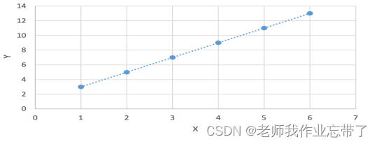
So when x=7 when , We forecast by 15.
- But usually , There is an approximate linear relationship between variables
| x | 1 | 2 | 3 | 4 | 5 | 6 |
| y | 3 | 2 | 8 | 8 | 11 | 13 |

The problem we have to solve is How to get a straight line can best explain the data ?
Fitting data
- Suppose there is only one dependent variable and independent variable , Each training example represents (𝑥𝑖 , 𝑦𝑖)
- use
 Indicates that according to the fitting line and x𝑖 Yes 𝑦𝑖 The predicted value of :
- Definition
 by Error term / residual
 Indicates that according to the fitting line and x𝑖 Yes 𝑦𝑖 The predicted value of :
 by
by A new definition is introduced here : Error term , It subtracts the estimated value of the sample from the true value of the sample .
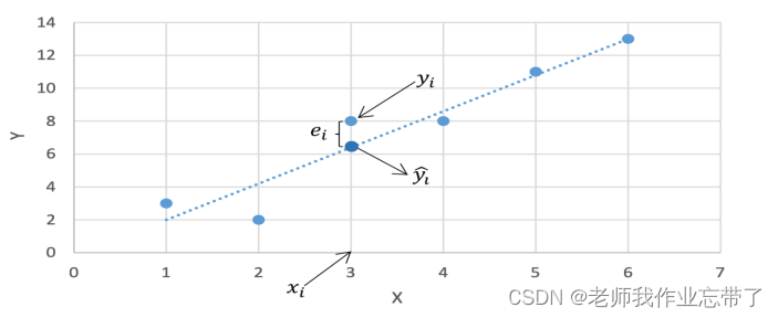
Our goal is Get a straight line so that the error term for all training samples is as small as possible
Basic assumptions of linear regression
We assume that :
- Suppose there is a relationship between the independent variable and the dependent variable linear relationship
- Between data points Independent
Output results y1,y2,y3... It doesn't matter.
- There is no collinearity between independent variables , Are independent of each other
Are you tired of walking : If the feature is The umbrella and a bag The two variables umbrella and schoolbag have nothing to do
If it is The weather The umbrella a bag be The weather and The umbrella We don't think they are independent
- Residual independence 、 Equivariance 、 accord with Normal distribution
error Independent 、 Equivariance ( Facing the same problem , It is also identically distributed )
according to Central limit theorem : Set from mean value to μ、 The variance of σ^2;( Co., LTD. ) The number of samples taken from any population is n The sample of , When n Sufficiently large , The sampling distribution of the sample mean value approximately follows that the mean value is μ、 The variance of σ^2/n Is a normal distribution .
3、 ... and 、 Loss function (loss function) The definition of
Various loss functions are feasible , You can think of it intuitively :
- Sum of all error terms
- The sum of the absolute values of all error terms
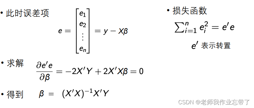
Considering optimization and other issues , The most common is Based on the sum of squares of errors Loss function of

• Using the sum of squares of errors as the loss function has many advantages
• The loss function is strictly convex , There is a unique solution
• The solution process is simple and easy to calculate
• At the same time, there are also some shortcomings
• The result is for “ outliers ”(outlier) Very sensitive
• resolvent : Detect outliers in advance and remove
• The loss function is equivalent for predictions that are above and below the true value
• But in some real cases, the impact of the two is different
We need to find the appropriate parameters b1、b2 Minimize the sum of squares of errors .
Least square method (Least Square, LS)
In order to solve the optimal intercept and slope , It can be transformed into a loss function Convex optimization problem , be called Least square method :
We are respectively right b1、b2 Finding partial derivatives :

This is the linear regression equation we recall at the beginning of this article , Of course, we don't have to calculate the partial derivative when we use it , Direct use .
Gradient descent method (Gradient Descent, GD)
Except least squares , The intercept and slope can also be updated iteratively with a gradient based method :
- You can initialize randomly first 𝑏1, 𝑏2
- repeat :


With an initialized set b1、b2, We can get the corresponding sample 1 The error term error1, Update based on the error term b,b=b-a, among a Is the update of the coefficient ( Function related to error , such as 0.1*error), In this way, there is a new b1、b2, Use a sample 2 The error term error2 Find out a Keep updating and iterating ... Until it converges .
Four 、 Multiple linear regression (Multiple Linear Regression)
When there are multiple dependent variables , We can express in matrix form
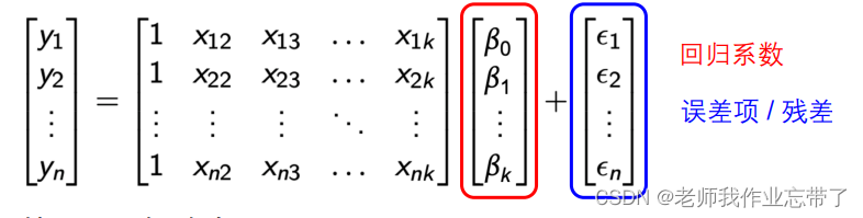
Based on the above matrix representation , Can be written as

here :
notes :
- matrix X The first column of is all 1, And β Multiplication means intercept .
- The result of the loss function is still a number
- Obtained by the least square method solve β Formula :


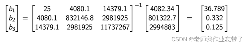
for example :
Recorded 25 Families are selling fast-moving goods and daily services every year
- The total cost (𝑌)
- Annual fixed income ( 𝑋2)、 Current assets held ( 𝑋3)
The following linear regression model can be built :

5、 ... and 、 The phase covariance of linear regression 、 Number of relationships 、 Coefficient of determination
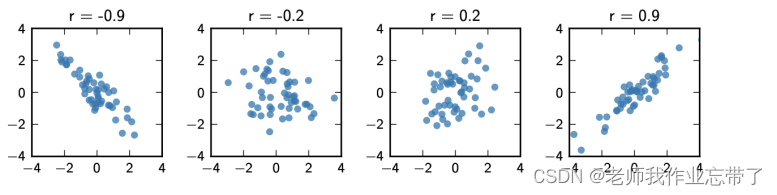
covariance : covariance , Describe two variables X and Y The degree of linear correlation

The correlation coefficient : Value range [-1,1]

Such as :
Coefficient of determination : Coefficient of determination  , Also called decision coefficient 、 Goodness of fit


Be careful : It may be less than 0, It is not the square of a number .
It measures the degree to which the model interprets the data
- y What percentage of fluctuations can be x Described by fluctuations in
- 𝑅 2 The closer the 1, It means that in regression analysis, the better the independent variable explains the dependent variable
Particular attention : Variable correlation ≠ There is a causal relationship
Prediction of comprehensive scores of World Universities Based on regression analysis
University ranking is a very important, challenging and controversial issue , The comprehensive strength of a university involves scientific research 、 Teachers' 、 Students and other aspects . At present, hundreds of evaluation institutions around the world will evaluate the comprehensive scores of universities to sort , And the scores of these institutions are often inconsistent . Among these rating agencies , World university ranking Center (Center for World University Rankings, abbreviation CWUR) To assess the quality of Education 、 Alumni employment 、 Research results and citations , Instead of relying on surveys and data submitted by universities , Is a very influential .
In this task, we will base on CWUR The ranking of famous universities around the world ( Teachers' 、 Scientific research, etc ), On the one hand, observe the characteristics of different universities through data visualization , On the other hand, I hope to build a machine learning model ( Linear regression ) Predict the comprehensive score of a University .
Data sources :World University Rankings | Kaggle
Data observation and processing :
import pandas as pd
import numpy as np

data_df = pd.read_csv('./cwurData.csv')
data_df.head(3).T # Observe the first few columns and transpose them for convenient observation 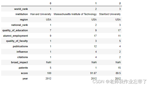
Remove the inclusion NaN The data of
data_df = data_df.dropna()
len(data_df) # 2000
Set up the matrix
feature_cols = ['quality_of_faculty', 'publications', 'citations', 'alumni_employment',
                'influence', 'quality_of_education', 'broad_impact', 'patents'] #  Extract eigenvalues
X = data_df[feature_cols]
Y = data_df['score']
# X Y They are independent variables   Dependent variable matrix
Data visualization
Observe the average scores of the top ten schools in the world , Therefore, we need to average the scores of the same school in different years . We can use groupby() function , Integrate the records of the same school and pass mean() The function averages . Then we sort them in descending order according to the average score , Take the top ten schools as the data to be observed .
import matplotlib.pyplot as plt
import seaborn as sns

mean_df = data_df.groupby('institution').mean()  #  Aggregate by school and average the aggregated columns
top_df = mean_df.sort_values(by='score', ascending=False).head(10)  #  Take the top ten schools
sns.set()
x = top_df['score'].values  #  Comprehensive score list
y = top_df.index.values  #  List of school names
sns.barplot(x, y, orient='h', palette="Blues_d")  #  Draw a bar chart
plt.xlim(75, 101)  #  Limit  x  Axis range
plt.show()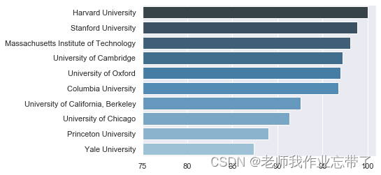
use pairplot Observe the correlation between variables , You can see from the figure , There is a linear relationship between a few variables ; Between variables and results , Approximate logarithmic relationship .
sns.pairplot(data_df[feature_cols + ['score']], height=3, diag_kind="kde")
plt.show()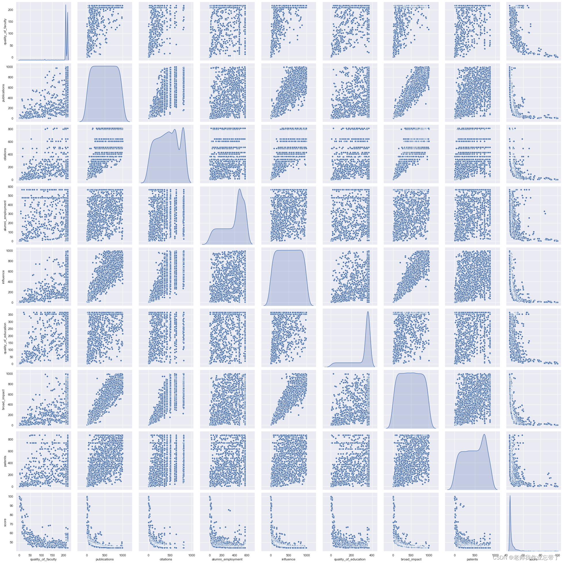
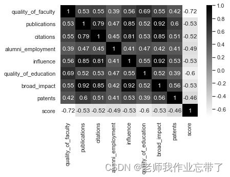
The correlation matrix can also be presented in the form of thermal diagram :
Build the model
Take out the columns of the corresponding independent variables and dependent variables , Then you can segment the training set and the test set based on this , And carry out model construction and analysis .
all_y = data_df['score'].values
all_x = data_df[feature_cols].values
#  take  values  It's to start from  pandas  Of  Series  Turn into  numpy  Of  array

from sklearn.model_selection import train_test_split
x_train, x_test, y_train, y_test = train_test_split(all_x, all_y, test_size=0.2, random_state=2020)
all_y.shape, all_x.shape, x_train.shape, x_test.shape, y_train.shape, y_test.shape #  Output data row and column information
# ((2000,), (2000, 8), (1600, 8), (400, 8), (1600,), (400,))
from sklearn.linear_model import LinearRegression
LR = LinearRegression() # linear regression model
LR.fit(x_train, y_train) # Train on the training set
p_test = LR.predict(x_test) # Predict on the test set , Obtain the predicted value
test_error = p_test - y_test # Prediction error
test_rmse = (test_error**2).mean()**0.5 # Calculation RMSE
'rmse: {:.4}'.format(test_rmse)
# rmse: 3.999Get the test set RMSE by 3.999, Calculate a fair result under the prediction goal of the percentage system . Judging from the evaluation indicators, it seems that we can estimate the comprehensive score according to the better ranking in all aspects , Next, let's observe the learned parameters , That is, the influence weight of each index ranking on the comprehensive score .
import matplotlib.pyplot as plt
import seaborn as sns

sns.set()
sns.barplot(x=LR.coef_, y=feature_cols)
plt.show()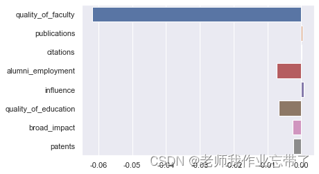
It will be found here that the prediction of comprehensive score is basically 「 The quality of teachers 」 This independent variable dominates ,「 employment 」 and 「 The quality of education 」 These two factors also have some influence , Other indicators play a small role .
To observe 「 The quality of teachers 」 The relationship between this dominant factor and the comprehensive score , We can go through seaborn Medium regplot() Function draws its distribution in the form of a scatter diagram .
sns.regplot(data_df['quality_of_faculty'], data_df['score'], marker="+")
plt.show()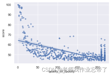
边栏推荐
- DNS series (I): why does the updated DNS record not take effect?
- SDNU_ ACM_ ICPC_ 2022_ Summer_ Practice(1~2)
- 韦东山第二期课程内容概要
- Deep dive kotlin collaboration (the end of 23): sharedflow and stateflow
- Reentrantlock fair lock source code Chapter 0
- 【愚公系列】2022年7月 Go教学课程 006-自动推导类型和输入输出
- 股票开户免费办理佣金最低的券商,手机上开户安全吗
- 5G NR 系统消息
- Thinkphp内核工单系统源码商业开源版 多用户+多客服+短信+邮件通知
- 【obs】Impossible to find entrance point CreateDirect3D11DeviceFromDXGIDevice
猜你喜欢
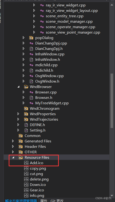
Qt添加资源文件,为QAction添加图标,建立信号槽函数并实现
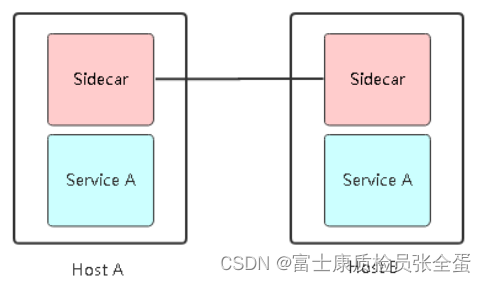
Service mesh introduction, istio overview
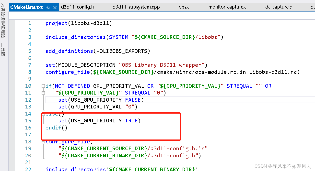
【obs】官方是配置USE_GPU_PRIORITY 效果为TRUE的
[OBS] the official configuration is use_ GPU_ Priority effect is true

They gathered at the 2022 ecug con just for "China's technological power"
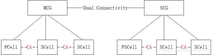
5g NR system messages
3 years of experience, can't you get 20K for the interview and test post? Such a hole?
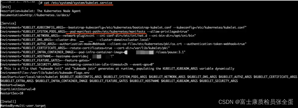
Kubernetes static pod (static POD)
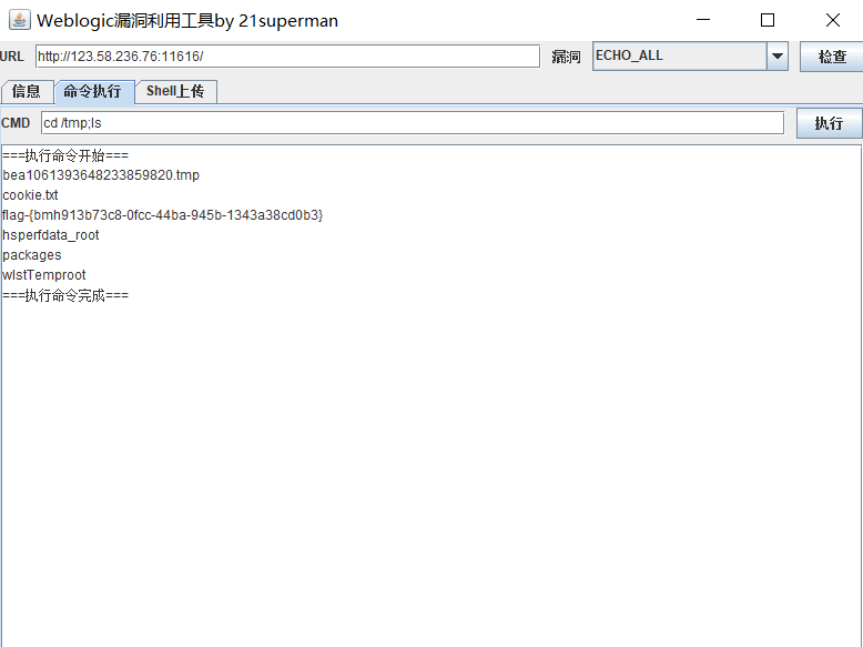
Fofa attack and defense challenge record

第四期SFO销毁,Starfish OS如何对SFO价值赋能?
随机推荐
韦东山第三期课程内容概要
From starfish OS' continued deflationary consumption of SFO, the value of SFO in the long run
新库上线 | CnOpenData中国星级酒店数据
股票开户免费办理佣金最低的券商,手机上开户安全吗
韦东山第二期课程内容概要
Reentrantlock fair lock source code Chapter 0
Cascade-LSTM: A Tree-Structured Neural Classifier for Detecting Misinformation Cascades(KDD20)
How to insert highlighted code blocks in WPS and word
Cve-2022-28346: Django SQL injection vulnerability
22年秋招心得
接口测试进阶接口脚本使用—apipost(预/后执行脚本)
Binder core API
服务器防御DDOS的方法,杭州高防IP段103.219.39.x
Basic types of 100 questions for basic grammar of Niuke
Basic mode of service mesh
[reprint] solve the problem that CONDA installs pytorch too slowly
Is it safe to open an account on the official website of Huatai Securities?
ReentrantLock 公平锁源码 第0篇
大数据开源项目,一站式全自动化全生命周期运维管家ChengYing(承影)走向何方?
Handwriting a simulated reentrantlock