当前位置:网站首页>Numerical analysis notes (I): equation root
Numerical analysis notes (I): equation root
2022-07-03 09:19:00 【fishfuck】
List of articles
Search of root
Step by step search
In a given interval [ a , b ] [a, b] [a,b] Up from the left endpoint x = a x=a x=a Start , In steps h h h Take it step by step f ( x 0 ) f(x_0) f(x0) and f ( x 0 + h ) f(x_0+h) f(x0+h), If found to be true f ( x 0 ) ⋅ f ( x 0 + h ) ≤ 0 f(x_0)\cdot f(x_0+h)\leq 0 f(x0)⋅f(x0+h)≤0 Then in the interval [ x 0 , x 0 + h ] [x_0,x_0+h] [x0,x0+h] Rooted .
When h h h Too many searches are required when it is too small , Too much calculation .
Two point search
Yes, there are root intervals [ a 0 , b 0 ] [a_0,b_0] [a0,b0] Implement the following dichotomy procedures : Midpoint x 0 = a 0 + b 0 2 x_0= \frac{a_0+b_0}2 x0=2a0+b0 Divide the interval into two halves , Judge the root x ∗ x^* x∗ stay x 0 x_0 x0 Which side of the road , So as to determine the new rooted interval [ a 1 , b 1 ] [a_1,b_1] [a1,b1], The length of [ a 0 , b 0 ] [a_0,b_0] [a0,b0] Half of . If the infinite loop goes on , There is a root interval It must be convergent At one point x ∗ x^* x∗.
Trial position method (Method of False Position
)thought : Looking for f ( a ) f(a) f(a) and f ( b ) f(b) f(b) Secant and x The intersection of the axes ( c , 0 ) (c,0) (c,0)
Iterative method
The core idea of iterative method is Explicit implicit equation . Put the equation f ( x ) = 0 f(x)=0 f(x)=0 to x = φ ( x ) x=\varphi (x) x=φ(x), Give an approximate value of the root of the equation x k x_k xk, Plug in , have to x k + 1 = φ ( x k ) x_{k+1}=\varphi (x_k) xk+1=φ(xk), That is, we can get the sequence starting from the given initial value x 1 , x 2 , x 3 , ⋯ x_1,x_2,x_3,\cdots x1,x2,x3,⋯. If this sequence is convergent , Then obviously there is the root of the equation x ∗ = lim k → ∞ x k x^*=\lim\limits_{k \to \infty}x_k x∗=k→∞limxk.
Judgment of convergence
If there is a neighborhood Δ : ∣ x − x ∗ ∣ ≤ δ , ∀ δ > 0 \Delta : |x-x^*|\leq\delta,\forall\delta>0 Δ:∣x−x∗∣≤δ,∀δ>0, In the iteration process ∀ x 0 ∈ Δ \forall x_0\in\Delta ∀x0∈Δ, It is called at the root x ∗ x^* x∗ Proximity convergence . among x 0 x_0 x0 Is the initial value of the iteration .
set up φ ( x ) \varphi(x) φ(x) In the equation x = φ ( x ) x=\varphi(x) x=φ(x) The root of the x ∗ x^* x∗ The neighborhood of has a continuous first derivative , And established ∣ φ ′ ( x ∗ ) ∣ < 1 |\varphi'(x^*)|<1 ∣φ′(x∗)∣<1, Then the iterative process x k + 1 = φ ( x k ) x_{k+1}=\varphi (x_k) xk+1=φ(xk) stay x ∗ x^* x∗ Proximity has local convergence . in other words , Iterative process with local convergence x k + 1 = φ ( x k ) x_{k+1}=\varphi (x_k) xk+1=φ(xk) For sufficiently accurate iterative initial values x ∗ x^* x∗ convergence .
Convergence rate
For iterative processes with local convergence x k + 1 = φ ( x k ) x_{k+1}=\varphi (x_k) xk+1=φ(xk), if φ ′ ( x ∗ ) ≠ 0 \varphi '(x^*)\neq0 φ′(x∗)=0 The iterative process is said to be linearly convergent , And when φ ′ ( x ∗ ) = 0 \varphi '(x^*)=0 φ′(x∗)=0 And φ ′ ′ ( x ∗ ) ≠ 0 \varphi ''(x^*)\neq0 φ′′(x∗)=0, The iterative process is said to be square convergent .
To accelerate the iteration
First, consider the linear iterative function
set up φ ( x ) \varphi (x) φ(x) Is a linear function φ ( x ) = L x + d , L > 0 \varphi (x)=Lx+d,L>0 φ(x)=Lx+d,L>0
Then the iterative formula of the given equation is x k + 1 = L x k + d x_{k+1}=Lx_k+d xk+1=Lxk+d
The root of the equation x ∗ x^* x∗ Satisfy x ∗ = L x ∗ + d x^*=Lx^*+d x∗=Lx∗+d
Subtracting two formulas , Yes x ∗ − x k + 1 = L ( x ∗ − x k ) x^*-x_{k+1}=L(x^*-x_k) x∗−xk+1=L(x∗−xk)
For iteration error e k = ∣ x ∗ − x k ∣ e_k=|x^*-x_k| ek=∣x∗−xk∣, Yes e k + 1 = L e k e_{k+1}=Le_k ek+1=Lek
Repeat , Yes e k = L k e 0 e_k=L^ke_0 ek=Lke0
L < 1 L<1 L<1 when , The iterative sequence converges , And L The smaller the size, the faster the convergence rate .
Use the above ideas , We can accelerate the iterative process . set up x k x_k xk It's a root x ∗ x^* x∗ An approximation of , Use the iterative formula to correct once , Yes x ˉ k + 1 = φ ( x k ) \bar{x}_{k+1}=\varphi(x_k) xˉk+1=φ(xk). hypothesis φ ′ ( x ) \varphi'(x) φ′(x) There is little change in the scope of investigation , Its estimated value is L L L, be x ∗ − x ˉ k + 1 ≈ L ( x ∗ − x k ) x^*-\bar{x}_{k+1}\approx L(x^*-x_k) x∗−xˉk+1≈L(x∗−xk). Find out x ∗ x^* x∗, Yes x ∗ ≈ 1 1 − L x ˉ k + 1 − L 1 − L x k x^*\approx\frac{1}{1-L}\bar{x}_{k+1}-\frac L{1-L}x_k x∗≈1−L1xˉk+1−1−LLxk. That is to say
{ x ˉ k + 1 = φ ( x k ) , Overlapping generation x K + 1 = 1 1 − L x ˉ k + 1 − L 1 − L x k , Add speed \left\{ \begin{array}{lr} \bar{x}_{k+1}=\varphi(x_k), & iteration \\ x_{K+1}=\frac{1}{1-L}\bar{x}_{k+1}-\frac L{1-L}x_k, & Speed up \\ \end{array} \right. { xˉk+1=φ(xk),xK+1=1−L1xˉk+1−1−LLxk, Overlapping generation Add speed
namely x k + 1 = 1 1 − L [ φ ( x k ) − L x k ] x_{k+1}=\frac1{1-L}[\varphi(x_k)-Lx_k] xk+1=1−L1[φ(xk)−Lxk]
However, the above accelerated iteration method needs to deal with the first derivative , It is not convenient for some iterative formulas . A more general , We have Aitken Acceleration method
{ x ˉ k + 1 = φ ( x k ) , Overlapping generation x ~ k + 1 = φ ( x ˉ k + 1 ) , Overlapping generation x K + 1 = x ~ k + 1 − ( x k + 1 − x ˉ k + 1 ) 2 x ~ k + 1 − 2 x ˉ k + 1 + x k , Add speed \left\{ \begin{array}{lr} \bar{x}_{k+1}=\varphi(x_k), & iteration \\ \tilde{x}_{k+1}=\varphi(\bar{x}_{k+1}),& iteration \\ x_{K+1}=\tilde{x}_{k+1}-\frac{(x_{k+1}-\bar{x}_{k+1})^2}{\tilde{x}_{k+1}-2\bar{x}_{k+1}+x_k}, & Speed up \\ \end{array} \right. ⎩⎪⎨⎪⎧xˉk+1=φ(xk),x~k+1=φ(xˉk+1),xK+1=x~k+1−x~k+1−2xˉk+1+xk(xk+1−xˉk+1)2, Overlapping generation Overlapping generation Add speed
The idea is to use the estimated value for the second iteration , Then do business to eliminate L L L, Finally, the solution is x ∗ x^* x∗, Just replace it .Aitken Its shortcomings are also obvious : It takes two iterations to get an estimate .
Newton Law ( Tangent method )
Newton method is the most widely used iterative method . The Newton formula is derived below . Investigate f ( x ) = 0 f(x)=0 f(x)=0, Let the approximate root be known x k x_k xk, Obviously , We hope that x k + 1 = x k + Δ x x_{k+1}=x_k+\Delta x xk+1=xk+Δx Try to satisfy f ( x k + Δ x ) ≈ 0 f(x_k+\Delta x)\approx0 f(xk+Δx)≈0. Replace its left end with its linear principal part , Yes f ( x k ) + f ′ ( x k ) Δ x = 0 f(x_k)+f'(x_k)\Delta x=0 f(xk)+f′(xk)Δx=0, thus , figure out Δ x = − f ( x k ) f ′ ( x k ) \Delta x=-\frac{f(x_k)}{f'(x_k)} Δx=−f′(xk)f(xk), Thus to x k + 1 = x k + Δ x x_{k+1}=x_k+\Delta x xk+1=xk+Δx Yes
x k + 1 = x k − f ( x k ) f ′ ( x k ) x_{k+1}=x_k-\frac{f(x_k)}{f'(x_k)} xk+1=xk−f′(xk)f(xk)
That's the famous one Newton Iterative formula
solve f ( x ) = x 2 − a = 0 f(x)=x^2-a=0 f(x)=x2−a=0 when , f ′ ( x ) = 2 x f'(x)=2x f′(x)=2x, Its Newton The iteration function is φ ( x ) = x − f ( x k ) f ′ ( x k ) = 1 2 ( a + a x ) \varphi(x)=x-\frac{f(x_k)}{f'(x_k)}=\frac{1}{2}\left(a+\frac ax\right) φ(x)=x−f′(xk)f(xk)=21(a+xa), This is the opening method of Ancient Mathematics .
Newton Improvement of the method
Newton How to go down the mountain
The basic idea : Each iteration ensures the descent condition , namely ∣ f ( x k + 1 ) ∣ < ∣ f ( x k ) ∣ |f(x_{k+1})|<|f(x_k)| ∣f(xk+1)∣<∣f(xk)∣, This ensures global convergence .
specific working means : Add the downhill factor λ \lambda λ, Will improve the value x k + 1 x_{k+1} xk+1 And the result of the previous step x k x_k xk Take the weighted average , namely x k + 1 = λ x ˉ k + 1 + ( 1 − λ ) x k x_{k+1}=\lambda \bar{x}_{k+1}+(1-\lambda)x_k xk+1=λxˉk+1+(1−λ)xk, That is to say , The iterative formula becomes x k + 1 = x k − λ f ( x k ) f ′ ( x k ) x_{k+1}=x_k-\lambda\frac{f(x_k)}{f'(x_k)} xk+1=xk−λf′(xk)f(xk), among λ \lambda λ Take from 1 Begin to λ \lambda λ Repeat and halve , Until you meet ∣ f ( x k + 1 ) ∣ < ∣ f ( x k ) ∣ |f(x_{k+1})|<|f(x_k)| ∣f(xk+1)∣<∣f(xk)∣.
String cutting
In order to avoid the calculation of derivatives , We can take secant instead of tangent , Thus, the iterative formula of chord cut method is derived : x k + 1 = x k − f ( x k ) f ( x k ) − f ( x 0 ) ( x k − x 0 ) x_{k+1}=x_k-\frac {f(x_k)}{f(x_k)-f(x_0)}(x_k-x_0) xk+1=xk−f(xk)−f(x0)f(xk)(xk−x0). Although the chord cut method avoids the calculation of derivatives , But its iteration speed is only one order .
Fast chord cut
To improve the efficiency of chord cutting , Then process the chord cutting formula , Thus, we derive the formula of fast chord cut method : x k + 1 = x k − f ( x k ) f ( x k ) − f ( x k − 1 ) ( x k − x k − 1 ) x_{k+1}=x_k-\frac {f(x_k)}{f(x_k)-f(x_{k-1})}(x_k-x_{k-1}) xk+1=xk−f(xk)−f(xk−1)f(xk)(xk−xk−1). The convergence speed of fast chord cut method is undoubtedly faster than that of chord cut method , But it needs to provide two iteration initial values , So it is also called two-step .
Improved Newton method
For the case of multiple roots , When f ( x ) = ( x − x ∗ ) m g ( x ) f(x)=(x-x^*)^mg(x) f(x)=(x−x∗)mg(x) And g ( x ∗ ) ≠ 0 g(x^*)\neq 0 g(x∗)=0 when , Directly use Newton's method , Its φ ′ ( x ∗ ) = 1 − 1 m > 0 \varphi '(x^*)=1-\frac 1m>0 φ′(x∗)=1−m1>0, It is only linear convergence .
One way to improve is to modify the iteration formula , elimination m m m, At this point, the iteration formula becomes φ ( x ) = x − m f ( x ) f ′ ( x ) \varphi (x)=x-m\frac{f(x)}{f'(x)} φ(x)=x−mf′(x)f(x), here φ ′ ( x ∗ ) = 0 \varphi '(x^*)=0 φ′(x∗)=0, Convergence becomes better . But this improvement method needs to know the specific order of multiple roots m m m.
Another way to improve is to use μ ( x ) = f ( x ) f ′ ( x ) \mu(x)=\frac{f(x)}{f'(x)} μ(x)=f′(x)f(x) And f ( x ) = ( x − x ∗ ) m g ( x ) f(x)=(x-x^*)^mg(x) f(x)=(x−x∗)mg(x) The nature of the same root , Yes μ ( x ) \mu(x) μ(x) Using Newton's method , φ ( x ) = x − μ ( x ) μ ′ ( x ) = x − f ( x ) f ′ ( x ) ∣ f ′ ( x ) ∣ 2 − f ( x ) f ′ ′ ( x ) \varphi(x)=x-\frac{\mu(x)}{\mu'(x)}=x-\frac{f(x)f'(x)}{|f'(x)|^2-f(x)f''(x)} φ(x)=x−μ′(x)μ(x)=x−∣f′(x)∣2−f(x)f′′(x)f(x)f′(x) Thus, the iterative formula is x k + 1 = x k − f ( x k ) f ′ ( x k ) ∣ f ′ ( x k ) ∣ 2 − f ( x k ) f ′ ′ ( x k ) x_{k+1}=x_k-\frac{f(x_k)f'(x_k)}{|f'(x_k)|^2-f(x_k)f''(x_k)} xk+1=xk−∣f′(xk)∣2−f(xk)f′′(xk)f(xk)f′(xk), It's easy to prove , It is second-order convergent .
边栏推荐
- The method of replacing the newline character '\n' of a file with a space in the shell
- 20220630 learning clock in
- AcWing 787. Merge sort (template)
- On a un nom en commun, maître XX.
- 【点云处理之论文狂读经典版13】—— Adaptive Graph Convolutional Neural Networks
- Jenkins learning (I) -- Jenkins installation
- 【点云处理之论文狂读经典版14】—— Dynamic Graph CNN for Learning on Point Clouds
- 浅谈企业信息化建设
- Digital management medium + low code, jnpf opens a new engine for enterprise digital transformation
- Bert install no package metadata was found for the 'sacraments' distribution
猜你喜欢

【Kotlin学习】类、对象和接口——定义类继承结构

Save the drama shortage, programmers' favorite high-score American drama TOP10
【点云处理之论文狂读经典版14】—— Dynamic Graph CNN for Learning on Point Clouds

Liteide is easy to use

What is an excellent fast development framework like?
Common penetration test range

推荐一个 yyds 的低代码开源项目
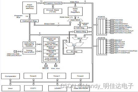
Pic16f648a-e/ss PIC16 8-bit microcontroller, 7KB (4kx14)

LeetCode 508. The most frequent subtree elements and

20220630 learning clock in
随机推荐
How to check whether the disk is in guid format (GPT) or MBR format? Judge whether UEFI mode starts or legacy mode starts?
[point cloud processing paper crazy reading cutting-edge version 12] - adaptive graph revolution for point cloud analysis
LeetCode 438. 找到字符串中所有字母异位词
Low code momentum, this information management system development artifact, you deserve it!
AcWing 786. 第k个数
【点云处理之论文狂读前沿版9】—Advanced Feature Learning on Point Clouds using Multi-resolution Features and Learni
2022-2-13 learn the imitation Niuke project - Project debugging skills
Methods of using arrays as function parameters in shell
Methods of checking ports according to processes and checking processes according to ports
Temper cattle ranking problem
AcWing 785. 快速排序(模板)
剑指 Offer II 029. 排序的循环链表
低代码起势,这款信息管理系统开发神器,你值得拥有!
Using variables in sed command
[point cloud processing paper crazy reading classic version 13] - adaptive graph revolutionary neural networks
Sword finger offer II 029 Sorted circular linked list
The method of replacing the newline character '\n' of a file with a space in the shell
【点云处理之论文狂读前沿版10】—— MVTN: Multi-View Transformation Network for 3D Shape Recognition
excel一小时不如JNPF表单3分钟,这样做报表,领导都得点赞!
【点云处理之论文狂读前沿版12】—— Adaptive Graph Convolution for Point Cloud Analysis