当前位置:网站首页>On data preprocessing in sklearn
On data preprocessing in sklearn
2022-07-02 12:00:00 【raelum】
Catalog
Preface
sklearn Medium sklearn.preprocessing The correlation function of data preprocessing is provided in , This article will mainly focus on feature scaling .
One 、 Standardization (StandardScaler)
Let the data matrix be
X = [ x 1 T x 2 T ⋮ x n T ] X= \begin{bmatrix} \boldsymbol{x}_1^{\mathrm T} \\ \boldsymbol{x}_2^{\mathrm T} \\ \vdots \\ \boldsymbol{x}_n^{\mathrm T} \end{bmatrix} X=⎣⎢⎢⎢⎡x1Tx2T⋮xnT⎦⎥⎥⎥⎤
among x i = ( x i 1 , x i 2 , ⋯ , x i d ) T \boldsymbol{x}_i=(x_{i1}, x_{i2},\cdots,x_{id})^{\mathrm T} xi=(xi1,xi2,⋯,xid)T Is the eigenvector .
Before proceeding to the next step , It is necessary to introduce the mean and standard deviation of the data matrix first .
We know , For data vectors a = ( a 1 , ⋯ , a n ) T \boldsymbol{a}=(a_1,\cdots,a_n)^{\mathrm T} a=(a1,⋯,an)T for ( The vector here can be understood as a set of data , It's called a vector , To facilitate subsequent statements ), The mean and standard deviation are :
μ ( a ) = a 1 + ⋯ + a n n , σ ( a ) = ( 1 n ∥ a − μ ( a ) ∥ 2 ) 1 / 2 , Its in μ ( a ) = ( μ ( a ) , ⋯ , μ ( a ) ⏟ n individual ) T \mu(\boldsymbol{a})=\frac{a_1+\cdots+a_n}{n},\quad\sigma(\boldsymbol a)=\left(\frac1n \Vert \boldsymbol{a}-\boldsymbol{\mu}(\boldsymbol{a})\Vert^2\right)^{1/2},\quad among \;\boldsymbol{\mu}(\boldsymbol{a})=(\underbrace{\mu(\boldsymbol{a}),\cdots, \mu(\boldsymbol{a})}_{n individual })^{\mathrm T} μ(a)=na1+⋯+an,σ(a)=(n1∥a−μ(a)∥2)1/2, Its in μ(a)=(n individual μ(a),⋯,μ(a))T
We will X X X Written as a line vector : X = ( a 1 , a 2 , ⋯ , a d ) X =(\boldsymbol{a}_1,\boldsymbol{a}_2,\cdots,\boldsymbol{a}_d) X=(a1,a2,⋯,ad), Each of them a i \boldsymbol{a}_i ai All vectors are columns , therefore
μ ( X ) = ( μ ( a 1 ) , μ ( a 2 ) , ⋯ , μ ( a d ) ) T σ ( X ) = ( σ ( a 1 ) , σ ( a 2 ) , ⋯ , σ ( a d ) ) T \begin{aligned} \mu(X)&=(\mu(\boldsymbol{a}_1),\mu(\boldsymbol{a}_2),\cdots,\mu(\boldsymbol{a}_d))^{\mathrm T} \\ \sigma(X)&=(\sigma(\boldsymbol{a}_1),\sigma(\boldsymbol{a}_2),\cdots,\sigma(\boldsymbol{a}_d))^{\mathrm T} \end{aligned} μ(X)σ(X)=(μ(a1),μ(a2),⋯,μ(ad))T=(σ(a1),σ(a2),⋯,σ(ad))T
Set right X X X After standardization, we get Z Z Z, utilize numpy The broadcast mechanism of , Z Z Z There are the following forms
Z = ( z 1 , z 2 , ⋯ , z d ) , Its in z i = a i − μ ( a i ) σ ( a i ) , i = 1 , 2 , ⋯ , d Z=(\boldsymbol{z}_1,\boldsymbol{z}_2,\cdots,\boldsymbol{z}_d),\quad among \; \boldsymbol{z}_i=\frac{\boldsymbol{a}_i-\mu(\boldsymbol{a}_i)}{\sigma(\boldsymbol{a}_i)},\;\;i=1,2,\cdots,d Z=(z1,z2,⋯,zd), Its in zi=σ(ai)ai−μ(ai),i=1,2,⋯,d
Of course Z Z Z Can be more succinctly expressed as
Z = X − μ ( X ) T σ ( X ) T Z=\frac{X-\mu(X)^{\mathrm T}}{\sigma(X)^{\mathrm T}} Z=σ(X)TX−μ(X)T
see X X X The average of , Variance and standard deviation :
from sklearn.preprocessing import StandardScaler
import numpy as np

#  Data matrix
X = np.array([
    [1, 3],
    [0, 1]
])
#  Create a scaler Instance and pass data into the instance
scaler = StandardScaler().fit(X)
#  see X Mean value of , Variance and standard deviation
print(scaler.mean_)  # [0.5 2. ]
print(scaler.var_)  # [0.25 1. ]
print(scaler.scale_)  # [0.5 1. ]
The reason why the standard deviation is scale_, Because our scaling standard is poor . It should be noted that , If the variance of a column of the data matrix is 0 0 0, be scale_ by 1 1 1, That is, this column is not scaled .
Yes X X X Standardize , Just use transfrom() Method :
X = np.array([
    [243, 80],
    [19, 47]
])
scaler = StandardScaler().fit(X)
#  Zoom
X_scaled = scaler.transform(X)
# [[ 1. 1.]
# [-1. -1.]]
see X_scaled Mean and standard deviation :
print(X_scaled.mean(axis=0))
# [0. 0.]
print(X_scaled.std(axis=0))
# [1. 1.]
You can see X_scaled The mean for 0 \boldsymbol 0 0, The standard deviation is 1 \boldsymbol 1 1, namely X X X It has been standardized .
Of course we can use scaler De standardizing new samples , The standardization process adopts X X X Mean and standard deviation :
X = np.array([
    [243, 80],
    [19, 47]
])
scaler = StandardScaler().fit(X)
#  Scale the new sample
print(scaler.transform([[2, 3]]))
# [[-1.15178571 -3.66666667]]
Two 、 normalization (MinMaxScaler)
Yes X X X Normalization is to normalize X X X Zoom all elements in to [ 0 , 1 ] [0,1] [0,1] Inside . The specific process is as follows :
remember
a i ‾ = min ( x 1 i , x 2 i , ⋯ , x n i ) , a i ‾ = max ( x 1 i , x 2 i , ⋯ , x n i ) X ‾ = ( a 1 ‾ , a 2 ‾ , ⋯ , a d ‾ ) T , X ‾ = ( a 1 ‾ , a 2 ‾ , ⋯ , a d ‾ ) T \underline{\boldsymbol{a}_i}=\min(x_{1i},x_{2i},\cdots,x_{ni}),\quad \overline{\boldsymbol{a}_i}=\max(x_{1i},x_{2i},\cdots,x_{ni}) \\ \\ \underline{X}=(\underline{\boldsymbol{a}_1},\underline{\boldsymbol{a}_2},\cdots,\underline{\boldsymbol{a}_d})^{\mathrm{T}},\quad \overline{X}=(\overline{\boldsymbol{a}_1},\overline{\boldsymbol{a}_2},\cdots,\overline{\boldsymbol{a}_d})^{\mathrm{T}} ai=min(x1i,x2i,⋯,xni),ai=max(x1i,x2i,⋯,xni)X=(a1,a2,⋯,ad)T,X=(a1,a2,⋯,ad)T
set up X X X After normalization, we get Z Z Z, utilize numpy The broadcast mechanism of , We have
Z = X − X ‾ T X ‾ T − X ‾ T Z=\frac{X-\underline{X}^{\mathrm T}}{\overline{X}^{\mathrm T}-\underline{X}^{\mathrm T}} Z=XT−XTX−XT
First use make_blobs() Generate speckle dataset :
from sklearn.preprocessing import MinMaxScaler
from sklearn.datasets import make_blobs

X, _ = make_blobs(n_samples=6, centers=2, random_state=27)
print(X)
# [[ 5.93412904 6.82960749]
# [-1.66484812 6.53450678]
# [-1.26216614 6.23733539]
# [ 5.26739446 7.73680694]
# [-0.66451524 7.50872847]
# [ 4.14680663 6.35238034]]
Yes X X X Normalize :
scaler = MinMaxScaler().fit(X)
print(scaler.transform(X))
# [[1. 0.39498722]
# [0. 0.19818408]
# [0.0529916 0. ]
# [0.91225996 1. ]
# [0.13164046 0.8478941 ]
# [0.76479434 0.07672366]]
If we want to X X X Zoom elements in to ( 1 , 2 ) (1, 2) (1,2) Within the interval , It only needs :
scaler = MinMaxScaler((1, 2)).fit(X)
print(scaler.transform(X))
# [[2. 1.39498722]
# [1. 1.19818408]
# [1.0529916 1. ]
# [1.91225996 2. ]
# [1.13164046 1.8478941 ]
# [1.76479434 1.07672366]]
3、 ... and 、 Regularization (Normalizer)
Yes X X X Regularization is to regularize each sample ( Every line ) Regularize , That is, the norm of each sample is transformed into the unit norm . The specific process is as follows :
x i : = x i ∥ x i ∥ p , i = 1 , 2 , ⋯ , n , p = 1 , 2 , ∞ \boldsymbol{x}_i:=\frac{\boldsymbol{x}_i}{\Vert \boldsymbol{x}_i\Vert_p},\quad i=1,2,\cdots,n,\quad p=1,2,\infty xi:=∥xi∥pxi,i=1,2,⋯,n,p=1,2,∞
p = 1 p=1 p=1 Time is L1 norm , p = 2 p=2 p=2 Time is L2 norm , p = ∞ p=\infty p=∞ Time is infinite ( Maximum ) norm .Normalizer By default L2 norm .
Yes X X X Conduct L2 Regularization :
from sklearn.preprocessing import Normalizer
import numpy as np

X = np.array([
    [1, 2, 3, 4],
    [5, 6, 7, 8]
])
scaler = Normalizer().fit(X)
print(scaler.transform(X))
# [[0.18257419 0.36514837 0.54772256 0.73029674]
# [0.37904902 0.45485883 0.53066863 0.60647843]]
If you want to use the maximum norm or L1 norm , It only needs :
scaler = Normalizer('max').fit(X)
print(scaler.transform(X))
# [[0.25 0.5 0.75 1. ]
# [0.625 0.75 0.875 1. ]]

scaler = Normalizer('l1').fit(X)
print(scaler.transform(X))
# [[0.1 0.2 0.3 0.4 ]
# [0.19230769 0.23076923 0.26923077 0.30769231]]
Four 、 Absolute maximum Standardization (MaxAbsScaler)
Yes X X X Normalize the absolute value maximum, that is, to X X X Each column of , Scale according to its maximum absolute value . The specific process is as follows :
remember
M a x A b s ( a i ) = max ( ∣ x 1 i ∣ , ∣ x 2 i ∣ , ⋯ , ∣ x n i ∣ ) , M a x A b s ( X ) = ( M a x A b s ( a 1 ) , ⋯ , M a x A b s ( a d ) ) T \mathrm{MaxAbs}(\boldsymbol{a_i})=\max(|x_{1i}|,|x_{2i}|,\cdots,|x_{ni}|),\quad \mathrm{MaxAbs}(X)=(\mathrm{MaxAbs}(\boldsymbol{a}_1),\cdots, \mathrm{MaxAbs}(\boldsymbol{a}_d))^{\mathrm T} MaxAbs(ai)=max(∣x1i∣,∣x2i∣,⋯,∣xni∣),MaxAbs(X)=(MaxAbs(a1),⋯,MaxAbs(ad))T
set up X X X After normalizing the absolute value, we get Z Z Z, utilize numpy The broadcast mechanism of , Yes
Z = X M a x A b s ( X ) T Z=\frac{X}{\mathrm{MaxAbs}(X)^{\mathrm T}} Z=MaxAbs(X)TX
Yes X X X Normalize the absolute maximum :
from sklearn.preprocessing import MaxAbsScaler
import numpy as np

X = np.array([
    [1, -1, 2],
    [2, 0, 0],
    [0, 1, -1]
])
scaler = MaxAbsScaler().fit(X)
print(scaler.transform(X))
# [[ 0.5 -1. 1. ]
# [ 1. 0. 0. ]
# [ 0. 1. -0.5]]
5、 ... and 、 Two valued (Binarizer)
Yes X X X Binarization is to set a threshold , X X X in Greater than The element of this threshold is set to 1 1 1, Less than or equal to The element of this threshold is set to 0 0 0.
Binarizer The default threshold is 0 0 0.
Yes X X X To binarize :
from sklearn.preprocessing import Binarizer
import numpy as np

X = np.array([
    [1, -1, 2],
    [2, 0, 0],
    [0, 1, -1]
])
transformer = Binarizer().fit(X)
print(transformer.transform(X))
# [[1 0 1]
# [1 0 0]
# [0 1 0]]
If the threshold is set to 1 1 1, Then the result becomes :
transformer = Binarizer(threshold=1).fit(X)
print(transformer.transform(X))
# [[0 0 1]
# [1 0 0]
# [0 0 0]]
in fact , utilize numpy Characteristics of , We can just use numpy Complete these operations :
import numpy as np

def binarizer(X, threshold):
    Y = X.copy()
    Y[Y > threshold] = 1
    Y[Y <= threshold] = 0
    return Y


X = np.array([
    [1, -1, 2],
    [2, 0, 0],
    [0, 1, -1]
])
print(binarizer(X, 0))
# [[1 0 1]
# [1 0 0]
# [0 1 0]]
边栏推荐
- MSI announced that its motherboard products will cancel all paper accessories
- Yygh-10-wechat payment
- Homer forecast motif
- Summary of flutter problems
- PyTorch中repeat、tile与repeat_interleave的区别
- 求16以内正整数的阶乘,也就是n的阶层(0=<n<=16)。输入1111退出。
- QT获取某个日期是第几周
- Pyqt5+opencv project practice: microcirculator pictures, video recording and manual comparison software (with source code)
- Thesis translation: 2022_ PACDNN: A phase-aware composite deep neural network for speech enhancement
- How to Add P-Values onto Horizontal GGPLOTS
猜你喜欢
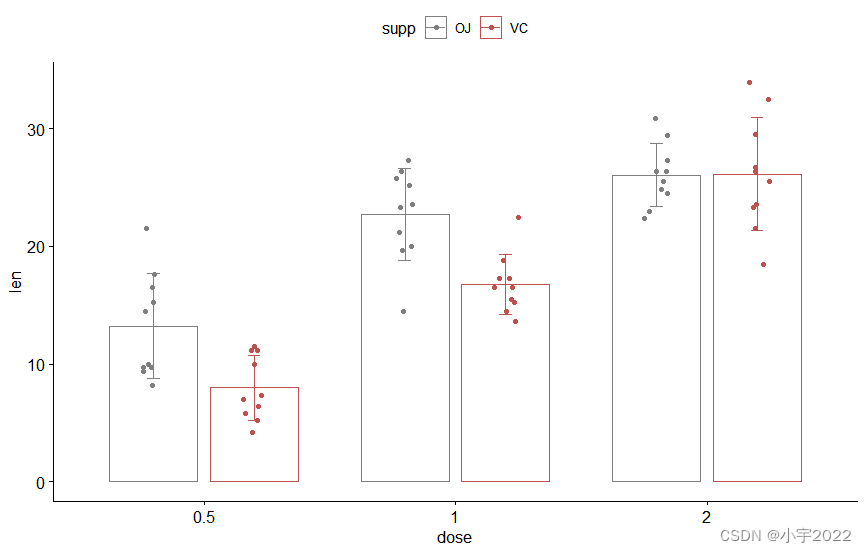
HOW TO EASILY CREATE BARPLOTS WITH ERROR BARS IN R

基于Arduino和ESP8266的连接手机热点实验(成功)
![[geek challenge 2019] upload](/img/04/731323142161a4994c14fedae38b81.jpg)
[geek challenge 2019] upload

多文件程序X32dbg动态调试
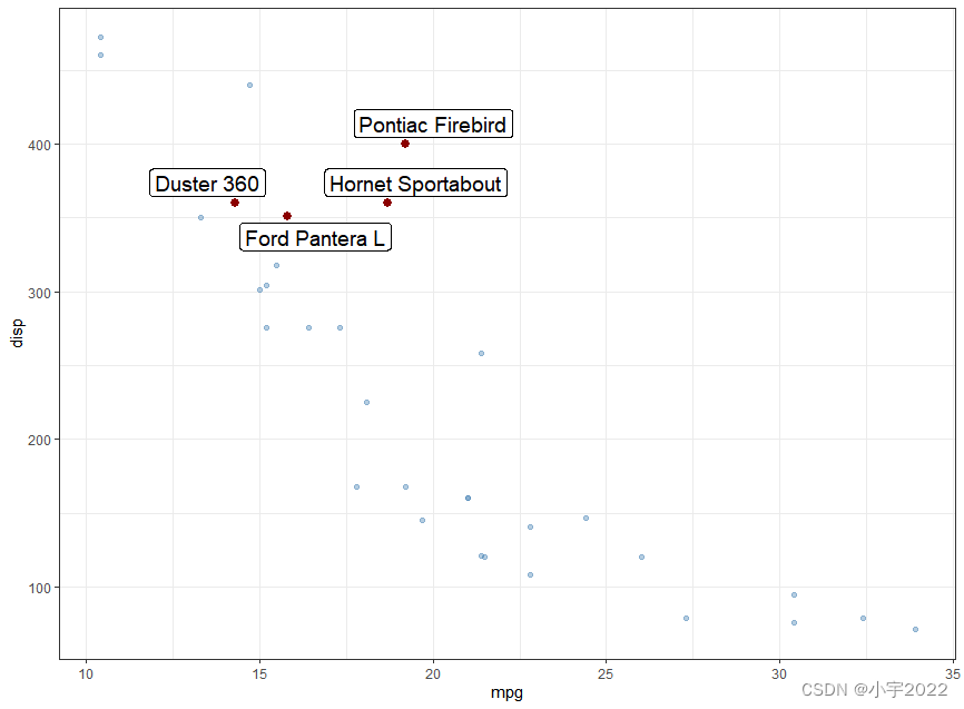
GGHIGHLIGHT: EASY WAY TO HIGHLIGHT A GGPLOT IN R

Dynamic memory (advanced 4)

文件操作(详解!)

【2022 ACTF-wp】

The position of the first underline selected by the vant tabs component is abnormal

The computer screen is black for no reason, and the brightness cannot be adjusted.
随机推荐
How to Create a Beautiful Plots in R with Summary Statistics Labels
PX4 Position_ Control RC_ Remoter import
Flesh-dect (media 2021) -- a viewpoint of material decomposition
文件操作(详解!)
QT获取某个日期是第几周
基于Arduino和ESP8266的Blink代码运行成功(包含错误分析)
Dynamic debugging of multi file program x32dbg
MySql存储过程游标遍历结果集
YYGH-BUG-04
Yygh-10-wechat payment
File operation (detailed!)
Analyse de l'industrie
How to Add P-Values onto Horizontal GGPLOTS
还不会安装WSL 2?看这一篇文章就够了
R HISTOGRAM EXAMPLE QUICK REFERENCE
Filtre de profondeur de la série svo2
Develop scalable contracts based on hardhat and openzeppelin (II)
SCM power supply
自然语言处理系列(一)——RNN基础
[visual studio 2019] create MFC desktop program (install MFC development components | create MFC application | edit MFC application window | add click event for button | Modify button text | open appl